Fourier Transform
The Fourier transform decomposes a function into different frequency components, which can be summed to represent the original function.
Fourier Series
TL;DR
- Any continuous periodic function can be represented by Fourier series, where Fourier coefficients are the weighted integrals of the periodic function over one period.
Definition
A periodic function $f_{T}(x)$ with a period $T$ can be decomposed into the following exponential form:
\[\begin{equation} f_{T}(x) = \sum_{n=-\infty}^{\infty} c_n e^{i 2\pi n \frac{x}{T}} \end{equation}\]where $c_n$ are Fourier coefficients:
\[\begin{equation} c_n = \frac{1}{T} \int_{T} f_{T}(x) e^{-i 2\pi n \frac{x}{T}} dx \end{equation}\]Continuous Fourier Transform
TL;DR
- The Fourier transform works for both periodic and non-periodic continuous functions.
- The Fourier transform is a special case of the Fourier series when the period goes to infinity.
- The Fourier transform of a periodic function is a summation of weighted delta functions at specific frequencies (harmonics of $1/T$), where the weights are the Fourier coefficients.
Definition
For any integrable real-valued function $f: \mathbb{R} \rightarrow \mathbb{C}$, the Fourier transform is defined as:
\[\begin{equation} \hat{f}(k) = \int_{-\infty}^{\infty} f(x) e^{-i 2\pi k x} dx \end{equation}\]where $k \in \mathbb{R}$ represents continuous frequencies. For example, if $x$ is measured in seconds, then frequency is in hertz. The Fourier transform is able to represent periodic and non-periodic functions, whereas the Fourier series only works for periodic functions.
The inverse Fourier transform is defined as:
\[\begin{equation} f(x) = \int_{-\infty}^{\infty} \hat{f}(k) e^{i 2\pi x k} dk \end{equation}\]$f(x)$ and $\hat{f}(k)$ are often referred to as a Fourier transform pair. Here, we use $\mathcal{F}$ and $\mathcal{F}^{-1}$ to denote the Fourier transform (FT) and inverse Fourier transform (iFT), respectively.
Sign of Fourier transform Remember the sign used in Fourier transform and inverse Fourier transform is just a convention. Mathematicians usually choose a negative sign for the inverse Fourier transform while engineers stuck to a positive sign for it. It is not that one is better than the other. The consistency is the key, otherwise errors and confusions may arise.
Connection to Fourier Series
Only periodic signals could be decomposed with Fourier series, what about non-periodic signals? We would see that Fourier transform is actually Fourier series when $T$ goes to the infinity, meaning there is non-periodic signals.
\[\begin{equation} \begin{split} f(x) &= \lim_{T \rightarrow \infty} f_T(x)\\ &= \lim_{T \rightarrow \infty} \sum_{n=-\infty}^{\infty} c_n e^{i 2\pi n \frac{x}{T}}\\ &= \lim_{T \rightarrow \infty} \sum_{n=-\infty}^{\infty} \left[ \frac{1}{T} \int_{T} f_{T}(x) e^{-i 2\pi n \frac{x}{T}} dx \right] e^{i 2\pi n \frac{x}{T}}\\ &= \lim_{\Delta{f_n} \rightarrow 0} \sum_{n=-\infty}^{\infty} \left[ \int_{-T/2}^{T/2} f_{T}(x) e^{-i 2\pi k_n x} dx \right] e^{i 2\pi x k_n} \Delta{k_n},\ k_n = \frac{n}{T}\ \Delta{k_n}=\frac{1}{T}\\ &= \int_{-\infty}^{\infty} \left[ \int_{-\infty}^{\infty} f(x) e^{-i 2\pi k x} dx \right] e^{i 2\pi x k} dk\\ &= \int_{-\infty}^{\infty} \hat{f}(k) e^{i 2\pi x k} dk \end{split} \end{equation}\]and that is exactly Fourier transform (note the definition of integral above).
Properties
Linearity
For any complex numbers $a$ and $b$, if $h(x)=af(x)+bg(x)$, then $\hat{h}(k) = \hat{f}(k) + \hat{g}(k)$.
Time Shifting
For any real number $x_0$, if $h(x)=f(x-x_0)$, then $\hat{h}(k)=e^{-i 2\pi x_0 k} \hat{f}(k)$.
\[\begin{equation} \begin{split} \mathcal{F}\left[h(x)\right] &= \int_{-\infty}^{\infty} f(x-x_0) e^{-i 2\pi k x} dx\\ &= \int_{-\infty}^{\infty} f(\hat{x}) e^{-i 2\pi k (\hat{x}+x_0)} d(\hat{x}+x_0)\\ &= e^{-i 2\pi x_0 k} \int_{-\infty}^{\infty} f(\hat{x}) e^{-i 2\pi k \hat{x}} d\hat{x}\\ &= e^{-i 2\pi x_0 k} \hat{f}(k) \end{split} \end{equation}\]Frequency Shifting
For any real number $k_0$, if $\hat{h}(k) = \hat{f}(k-k_0)$, then $h(x)=e^{i 2 \pi k_0 x} f(x)$.
\[\begin{equation} \begin{split} \mathcal{F}^{-1}\left[\hat{h}(k)\right] &= \int_{-\infty}^{\infty} \hat{f}(k-k_0) e^{i 2\pi x k} dk\\ &= \int_{-\infty}^{\infty} \hat{f}(\hat{k}) e^{i 2\pi x(\hat{k}+k_0)} d(\hat{k}+k_0)\\ &= e^{i 2\pi k_0 x} \int_{-\infty}^{\infty} \hat{f}(\hat{k}) e^{i 2\pi x\hat{k}} d\hat{k}\\ &= e^{i 2\pi k_0 x} f(x) \end{split} \end{equation}\]Scale Property
For any real number $a$, if $h(x)=f(ax)$, then $\hat{h}(k)=\frac{1}{|a|}\hat{f}(\frac{k}{a})$. Let’s assuming $a \gt 0$:
\[\begin{equation} \begin{split} \mathcal{F}\left[h(x)\right] &= \int_{-\infty}^{\infty} f(ax) e^{-i 2\pi k x} dx\\ &= \int_{-\infty}^{\infty} f(\hat{x}) e^{-i 2\pi k (\hat{x}/a)} d(\hat{x}/a)\\ &= \frac{1}{a} \int_{-\infty}^{\infty} f(\hat{x}) e^{-i 2\pi (k / a) \hat{x}} d\hat{x}\\ &= \frac{1}{a} \hat{f}(\frac{k}{a}) \end{split} \end{equation}\]and if $a \lt 0$:
\[\begin{equation} \begin{split} \mathcal{F}\left[h(x)\right] &= \int_{-\infty}^{\infty} f(ax) e^{-i 2\pi k x} dx\\ &= \int_{\infty}^{-\infty} f(\hat{x}) e^{-i 2\pi k (\hat{x}/a)} d(\hat{x}/a)\\ &= \frac{1}{-a} \int_{-\infty}^{\infty} f(\hat{x}) e^{-i 2\pi (k/ a) \hat{x}} d\hat{x}\\ &= \frac{1}{-a} F(\frac{k}{a}) \end{split} \end{equation}\]Time Convolution Theorem
For Fourier transform pairs $f(x) \leftrightarrow \hat{f}(k)$ and $g(x) \leftrightarrow \hat{g}(k)$, we have:
\[\begin{equation} \begin{split} \mathcal{F}\left[f(x) \ast g(x)\right] &= \int_{-\infty}^{\infty} \int_{-\infty}^{\infty} f(\tau)g(x-\tau) d\tau e^{-i 2\pi k x} dx \\ &= \int_{-\infty}^{\infty} \int_{-\infty}^{\infty} g(x-\tau) e^{-i 2\pi k x} dx f(\tau) d\tau\\ &= \int_{-\infty}^{\infty} \int_{-\infty}^{\infty} g(\hat{x}) e^{-i 2\pi k (\hat{x}+\tau)} d(\hat{x}+\tau) f(\tau) d\tau\\ &= \int_{-\infty}^{\infty} \left(\int_{-\infty}^{\infty} g(\hat{x}) e^{-i 2\pi k \hat{x}} d\hat{x}\right) f(\tau) e^{-i 2\pi k \tau} d\tau\\ &= \hat{g}(k) \int_{-\infty}^{\infty} f(\tau) e^{-i 2\pi k \tau} d\tau\\ &= \hat{g}(k) \hat{f}(k) \end{split} \end{equation}\]Frequency Convolution Theorem
For Fourier transform pairs $f(x) \leftrightarrow \hat{f}(k)$ and $g(x) \leftrightarrow \hat{g}(k)$, we have:
\[\begin{equation} \begin{split} \mathcal{F}^{-1}\left[\hat{f}(k) \ast \hat{g}(k)\right] &= \int_{-\infty}^{\infty} \int_{-\infty}^{\infty} \hat{f}(\tau) \hat{g}(k-\tau) d\tau e^{i 2\pi x k} dk\\ &= \int_{-\infty}^{\infty} \int_{-\infty}^{\infty} \hat{g}(k-\tau) e^{i 2\pi x k} dk \hat{f}(\tau) d\tau\\ &= \int_{-\infty}^{\infty} \int_{-\infty}^{\infty} \hat{g}(\hat{k}) e^{i 2\pi x (\hat{k}+\tau)} d(\hat{k}+\tau) \hat{f}(\tau) d\tau\\ &= \int_{-\infty}^{\infty} \left(\int_{-\infty}^{\infty} \hat{g}(\hat{k}) e^{i 2\pi x \hat{k}} d\hat{k}\right) \hat{f}(\tau) e^{i 2\pi x \tau} d\tau\\ &= g(x) \int_{-\infty}^{\infty} \hat{f}(\tau) e^{i 2\pi x \tau} d\tau\\ &= g(x) f(x) \end{split} \end{equation}\]Conguation
\[\begin{equation} \begin{split} \mathcal{F}\left[\overline{f(x)}\right] &= \int_{-\infty}^{\infty} \overline{f(x)} e^{-i 2\pi k x} dx \\ &= \overline{ \int_{-\infty}^{\infty} f(x) e^{i 2\pi k x} dx}\\ &= \overline{ \int_{-\infty}^{\infty} f(x) e^{-i 2\pi (-k) x} dx}\\ &= \overline{\hat{f}(-k)} \end{split} \end{equation}\]If $f(x)$ is a real-valued function, then $\hat{f}(-k)=\overline{\hat{f}(k)}$, which is referred to as conjugate symmetric property. If $f(x)$ is an imaginary-valued function, then $\hat{f}(-k)=- \overline{\hat{f}(k)}$, which is referred to as conjugate anti-symmetric property. Same properties occur in the inverse Fourier transform.
Common FT Pairs
| Time Domain | Frequency Domain | Description |
|---|---|---|
| $1$ | $\delta(k)$ | $\delta(k) = \int_{-\infty}^{\infty} e^{-i 2\pi k x} dx$ |
| $\delta(x)$ | $1$ | $1 = \int_{-\infty}^{\infty} \delta(x) e^{-i 2\pi k x} dx$ |
| $\mathrm{sgn}(x) = { 1 \text{ if } x > 0,\ 0 \text{ if } x = 0,\ -1 \text{ if } x < 0 }$ | $\mathrm{sgn}(x)$ is the sign function | |
| $u(x) = {1 \text{ if } x \gt 0,\ 1/2 \text{ if } x = 0,\ 0 \text{ if } x \lt 0}$ | $\frac{1}{2}\left(\delta(k) + 1/(i\pi k)\right)$ | $u(x)$ is the unit step function. $u(x)=\frac{1}{2}(1+\mathrm{sgn}(x))$ |
| $e^{i a x}$ | $\delta(k-a/(2\pi))$ | Frequency Shifting |
| $\mathrm{cos}(ax)$ | $\frac{1}{2}\left(\delta(k-a/(2\pi)) + \delta(k+a/(2\pi))\right)$ | $\mathrm{cos}(ax) =\ \frac{1}{2}(e^{i a x} + e^{-i a x})$ |
| $\mathrm{sin}(ax)$ | $\frac{1}{2}\left(\delta(k-a/(2\pi)) - \delta(k+a/(2\pi))\right)$ | $\mathrm{sin}(ax) =\ \frac{1}{2}(e^{i a x} - e^{-i a x})$ |
| $\mathrm{rect}(x)={ 1 \text{ if } \lvert x \rvert \lt 1/2,\ 1/2 \text{ if } \lvert x \rvert = 1/2,\ 0 \text{ if } \lvert x \rvert \gt 1/2 }$ | $\mathrm{sinc}(k) = \mathrm{sin}(\pi k)/(\pi k)$ | $\mathrm{rect}(x) =\ u(x+1/2)-u(x-1/2)$ |
| $\mathrm{sinc}(x)$ | $\mathrm{rect}(k)={1 \text{ if } \lvert k \rvert \lt 1/2,\ 1/2 \text{ if } \lvert k \rvert = 1/2,\ 0 \text{ if } \lvert k \rvert \gt 1/2 } $ | |
| $\sum_{n=-\infty}^{\infty} \delta(x-n \Delta x)$ | $\frac{1}{\Delta x} \sum_{m=-\infty}^{\infty} \delta(k-m/\Delta x)$ | Comb function |
Comb Function
A comb function (a.k.a sampling function, sometimes referred to as impulse sampling) is a periodic function with the formula:
\[\begin{equation} S_{\Delta{x}}(x) = \sum_{n=-\infty}^{\infty} \delta(x-n\Delta{x}) \end{equation}\]where $\Delta{x}$ is the given period. Fourier transform could be extended to [[generalized functions]] like $\delta(x)$, which makes it possible to bypass the limitation of absolute integrable property on $f(x)$. The key is to decompose periodic functions into Fourier series and use additive property of Fourier transform .
The Fourier transform of $S_{\Delta{x}}(x)$ is:
\[\begin{equation} \begin{split} \mathcal{F}\left(S_{\Delta{x}}(x)\right) &= \int_{-\infty}^{\infty} \sum_{n=-\infty}^{\infty} \delta(x-n\Delta{x}) e^{-i 2\pi k x} dx\\ &= \sum_{n=-\infty}^{\infty} \int_{-\infty}^{\infty} \delta(x-n\Delta{x}) e^{-i 2\pi k x} dx\\ &= \sum_{n=-\infty}^{\infty} e^{-i 2\pi k n \Delta{x}}\\ \end{split} \end{equation}\]It is not obvious to see what the transform is, but we can prove it with Fourier series. Note that $S_{\Delta{x}}(x)$ is a periodic function, its Fourier series is represented as:
\[\begin{equation} \begin{split} c_n &= \frac{1}{\Delta{x}} \int_{\Delta{x}} S_{\Delta{x}}(x) e^{-i 2\pi n x / \Delta{x}} dx\\ &= \frac{1}{\Delta{x}} \int_{-\frac{\Delta{x}}{2}}^{\frac{\Delta{x}}{2}} \sum_{m=-\infty}^{\infty} \delta(x-m\Delta{x}) e^{-i 2\pi n x / \Delta{x}} dx\\ &= \frac{1}{\Delta{x}} \int_{-\frac{\Delta{x}}{2}}^{\frac{\Delta{x}}{2}} \delta(x) e^{-i 2\pi n x / \Delta{x}} dx\\ &= \frac{1}{\Delta{x}} \int_{-\infty}^{\infty} \delta(x) e^{-i 2\pi n x / \Delta{x}} dx\\ &= \frac{1}{\Delta{x}}\\ S_{\Delta{x}}(x) &= \sum_{n=-\infty}^{\infty} c_n e^{i 2\pi n x / \Delta{x}}\\ &= \frac{1}{\Delta{x}} \sum_{n=-\infty}^{\infty} e^{i 2\pi n x / \Delta{x}} \end{split} \end{equation}\]and Dirac delta function is expressed as:
\[\begin{equation} \begin{split} \delta(x) &= \int_{-\infty}^{\infty} e^{i 2\pi x k} dk\\ &= \int_{-\infty}^{\infty} e^{-i 2\pi x (-k)} dk\\ &= \int_{\infty}^{-\infty} e^{-i 2\pi x \hat{k}} d(-\hat{k})\\ &= \int_{-\infty}^{\infty} e^{-i 2\pi x \hat{k}} d(\hat{k}) \end{split} \end{equation}\]Now we can apply Fourier transform to $S_{\Delta{x}}(x)$:
\[\begin{equation} \begin{split} \mathcal{F}\left(S_{\Delta{x}}(x)\right) &= \int_{-\infty}^{\infty} \sum_{n=-\infty}^{\infty} c_n e^{i 2\pi n x / \Delta{x}} e^{-i 2\pi k x} dx\\ &= \frac{1}{\Delta{x}} \sum_{n=-\infty}^{\infty} \int_{-\infty}^{\infty} e^{i 2\pi (n/\Delta{x} - k) x} dx\\ &= \frac{1}{\Delta{x}} \sum_{n=-\infty}^{\infty} \delta({k - n/\Delta{x}}) \end{split} \end{equation}\]so $\mathcal{F}\left(S_{\Delta{x}}(x)\right)$ is also a periodic function with the period as $1/\Delta{x}$. Hence, we again apply Fourier series:
\[\begin{equation} \begin{split} c_n &= \Delta{x} \int_{\frac{1}{\Delta{x}}} \mathcal{F}\left(S_{\Delta{x}}(x)\right) e^{-i 2\pi n k \Delta{x}} dk\\ &= \int_{-\frac{1}{2\Delta{x}}}^{\frac{1}{2\Delta{x}}} \sum_{m=-\infty}^{\infty} \delta(k-m/\Delta{x}) e^{-i 2\pi n k \Delta{x}} dk\\ &= \int_{-\frac{1}{2\Delta{x}}}^{\frac{1}{2\Delta{x}}} \delta(k) e^{-i 2\pi n k \Delta{x}} dk\\ &= \int_{-\infty}^{\infty} \delta(k) e^{-i 2\pi n k \Delta{x}} dk\\ &= 1\\ \mathcal{F}\left(S_{\Delta{x}}(x)\right) &= \sum_{n=-\infty}^{\infty} c_n e^{i 2\pi n k \Delta{x}}\\ &= \sum_{n=-\infty}^{\infty} e^{i 2\pi n k \Delta{x}}\\ &= \sum_{n=-\infty}^{\infty} e^{-i 2\pi n k \Delta{x}} \end{split} \end{equation}\]and we can see that why Fourier transform of a comb function is still a comb function.
FT of Periodic Functions
With the help of Dirac delta function, Fourier transform could also be used on periodic functions. Considering a periodic function $f_{T}(x)$ with period $T$, we can write it as a Fourier series:
\[\begin{equation} f_{T}(x) = \sum_{n=-\infty}^{\infty} c_n e^{i 2\pi n x/T} \end{equation}\]Let’s compute the Fourier transform:
\[\begin{equation} \begin{split} \mathcal{F}(f_T(x)) &= \int_{-\infty}^{\infty} f_T(x) e^{-i 2\pi k x} dx\\ &= \sum_{n=-\infty}^{\infty} c_n \int_{-\infty}^{\infty} e^{i 2\pi (n/T-k) x} dx\\ &= \sum_{n=-\infty}^{\infty} c_n \delta(n/T - k)\\ &= \sum_{n=-\infty}^{\infty} c_n \delta(k - n/T) \end{split} \end{equation}\]so the Fourier transform of a periodic function is a sum of delta functions at the Fourier series frequencies and the weight of each delta function is the Fourier series coefficient, as we proved in the Fourier transform of the comb function.
The inverse Fourier transform is:
\[\begin{equation} \begin{split} \mathcal{F}(\sum_{n=-\infty}^{\infty} c_n \delta(k - n/T)) &= \int_{-\infty}^{\infty} \sum_{n=-\infty}^{\infty} c_n \delta(k - n/T) e^{i 2\pi x k} dk\\ &= \sum_{n=-\infty}^{\infty} c_n \int_{-\infty}^{\infty} \delta(k - n/T) e^{i 2\pi x k} dk\\ &= \sum_{n=-\infty}^{\infty} c_n e^{i 2\pi x n/T}\\ &= f_T(x) \end{split} \end{equation}\]Discrete-Time Fourier Transform
TL;DR
- The discrete-time Fourier transform (DTFT) is a special case of the Fourier transform when the original function is sampled.
- The frequency domain of DTFT is continuous but periodic, with a period of $1/\Delta{x}$, where $\Delta{x}$ is the sampling interval.
- The DTFT of periodic sequence is a summation of weighted delta functions.
Definition
For a discrete sequence of real or complex values $f[n]$ with all integers $n$, the discrete-time Fourier transform is defined as:
\[\begin{equation} \hat{f}_{dtft}(k) = \sum_{n=-\infty}^{\infty} f[n] e^{-i2\pi n k \Delta{x}} \end{equation}\]where $\frac{1}{\Delta{x}}$ is the sampling frequency in the time domain. This formula can be seen as a Fourier series ($-$ and $+$ signs are the same thing) and $\hat{f}_{dtft}(k)$ is actually a periodic function with period $1/\Delta{x}$.
The inverse discrete-time Fourier transform is defined as:
\[\begin{equation} f[n] = \Delta{x} \int_{1/\Delta{x}} \hat{f}_{dtft}(k) e^{i 2\pi n k \Delta{x}} dk \end{equation}\]note the integral is only evaluated in a period.
Here we use $\mathcal{F}_{dtft}$ to represent the discrete-time Fourier transform (DTFT), and $\mathcal{F}_{dtft}^{-1}$ to represent the inverse discrete-time Fourier transform (iDTFT).
Connection to the FT
Modern computers can only handle discrete values instead of continuous signals. The most basic discretization technique is sampling. Considering a continuous function $f(x)$ and an uniform sampling pattern $S_{\Delta{x}}(x) = \sum_{n=-\infty}^{\infty} \delta(x-n\Delta{x})$, which is the Comb Function we described above, the sampling process can be simulated as:
\[\begin{equation} \begin{split} f_S(x) &= f(x) S_{\Delta{x}}(x)\\ &= \sum_{n=-\infty}^{\infty} f(x)\delta(x-n\Delta{x}) \end{split} \end{equation}\]The Fourier transform (using the definition) of the above function is:
\[\begin{equation} \begin{split} \hat{f}_S(k) &= \int_{-\infty}^{\infty} f_S(x) e^{-i 2\pi k x} dx\\ &= \int_{-\infty}^{\infty} \left( \sum_{n=-\infty}^{\infty} f(x)\delta(x-n\Delta{x}) \right) e^{-i 2\pi k x} dx\\ &= \sum_{n=-\infty}^{\infty} \left( \int_{-\infty}^{\infty} f(x) e^{-i 2\pi k x} \delta(x-n\Delta{x}) dx\right)\\ &= \sum_{n=-\infty}^{\infty} f(n\Delta{x})e^{-i 2\pi k n\Delta{x}},\ f[n]=f(n\Delta{x})\\ &=\sum_{n=-\infty}^{\infty} f[n] e^{-i 2\pi n k \Delta{x}}\\ &= \hat{f}_{dtft}(k) \end{split} \end{equation}\]which is the definition of discrete-time Fourier transform. The next step is to prove the correctness of the inverse discrete-time Fourier transform:
\[\begin{equation} \begin{split} \Delta{x} \int_{1/\Delta{x}} \hat{f}_{dtft}(k) e^{i 2\pi n k \Delta{x}} dk &= \Delta{x} \int_{-\frac{1}{2\Delta{x}}}^{\frac{1}{2\Delta{x}}} \hat{f}_{dtft}(k) e^{i 2\pi n k \Delta{x}} dk\\ &= \Delta{x} \int_{-\frac{1}{2\Delta{x}}}^{\frac{1}{2\Delta{x}}} \hat{f}_{S}(k) e^{i 2\pi n k \Delta{x}} dk\\ &=\Delta{x} \int_{-\frac{1}{2\Delta{x}}}^{\frac{1}{2\Delta{x}}} \left[\sum_{m=-\infty}^{\infty} f[m] e^{-i 2\pi m k \Delta{x}}\right] e^{i 2\pi n k \Delta{x}} dk\\ &=\Delta{x} \sum_{m=-\infty}^{\infty} f[m] \left[ \int_{-\frac{1}{2\Delta{x}}}^{\frac{1}{2\Delta{x}}} e^{i 2\pi (n-m) k \Delta{x}} dk \right]\\ &= \Delta{x} \sum_{m=-\infty}^{\infty} f[m] \left[ \left. \frac{1}{i 2\pi (n-m) \Delta{x}} e^{i 2\pi (n-m) k \Delta{x}} \right|_{-\frac{1}{2\Delta{x}}}^{\frac{1}{2\Delta{x}}} \right]\\ &= \Delta{x} \sum_{m=-\infty}^{\infty} f[m] \left[\frac{1}{\Delta{x}} \frac{\sin(\pi(n-m))}{\pi (n-m)}\right]\\ &= f[n] \end{split} \end{equation}\]note that $\mathrm{sinc}(x)=\frac{\sin(\pi x)}{\pi x}$ only has a nonzero value 1 at $x=0$ and 0 for other integers.
It is clear that $\hat{f}_S(k)$ is a periodic function with period $1/\Delta{x}$, we can see that from the convolution theorem of the Fourier transform:
\[\begin{equation} \begin{split} \hat{f}_S(k) &= \mathcal{F}\left[f(x)S_{\Delta{x}}(x)\right]\\ &= \mathcal{F}\left[f(x)\right] \ast \mathcal{F}\left[S_{\Delta{x}}(x)\right]\\ &= \hat{f}(k) \ast \hat{S}_{\Delta{x}}(k)\\ &= \hat{f}(k) \ast \frac{1}{\Delta{x}} \sum_{n=-\infty}^{\infty} \delta(k - n/\Delta{x})\\ &= \frac{1}{\Delta{x}} \sum_{n=-\infty}^{\infty} \hat{f}(k) \ast \delta(k - n/\Delta{x})\\ &= \frac{1}{\Delta{x}} \sum_{n=-\infty}^{\infty} \int_{-\infty}^{\infty} \hat{f}(\tau) \delta(k - \tau - n/\Delta{x}) d\tau\\ &= \frac{1}{\Delta{x}} \sum_{n=-\infty}^{\infty} \int_{-\infty}^{\infty} \hat{f}(\tau) \delta(-(\tau - k + n/\Delta{x})) d\tau\\ &= \frac{1}{\Delta{x}} \sum_{n=-\infty}^{\infty} \int_{-\infty}^{\infty} \hat{f}(\tau) \delta(\tau - (k - n/\Delta{x})) d\tau\\ &= \frac{1}{\Delta{x}} \sum_{n=-\infty}^{\infty} \hat{f}(k-n/\Delta{x})\\ \end{split} \end{equation}\]so the discrete-time Fourier transform of $f[n]$ is a summation of shifted replicates of $\hat{f}(k)$ in terms of a frequency period $1/\Delta{x}$.
Common DTFT Pairs
DTFT of Periodic Sequences
Considering $f[n]$ is an $N$-periodic sequence, we can write $f[n]$ as $f_S(x) = f_T(x) S_{\Delta{x}}(x)$, where $N\Delta{x}=T$. $f_S(x)$ is also a periodic function with a period $T$:
\[\begin{equation} \begin{split} f_{S}(x+T) &= f_{T}(x+T) S_{\Delta{x}}(x+T)\\ &= f_T(x) S_{\Delta{x}}(x+N\Delta{x})\\ &= f_T(x) S_{\Delta{x}}(x)\\ &= f_S(x)\\ f[n+N] &= f_S((n+N)\Delta{x})\\ &= f_S(n\Delta{x}+T)\\ &= f_S(n\Delta{x})\\ &= f[n] \end{split} \end{equation}\]For delta function, we also know that:
\[\begin{equation} \begin{split} \int_{a}^{b} f(x) \delta(x-x_0) dx &=\\ &= \int_{-\infty}^{\infty} f(x) \left(u(x-a) - u(x-b)\right) \delta(x-x_0) dx\\ &= f(x_0)\left(u(x_0-a) - u(x_0-b)\right)\\ &= \begin{cases} f(x_0) & x_0 \in (a, b)\\ f(x_0)/2 & x_0=a,b\\ 0 & \text{else} \end{cases} \end{split} \end{equation}\]where $u(x)$ is the unit step function.
Remember that Fourier transform of a periodic function is a summation of delta functions weighted by the Fourier coefficients:
\[\begin{equation} \begin{split} c_m &= \frac{1}{T} \int_{T} f_{S}(x) e^{-i 2\pi m x / T} dx\\ &= \frac{1}{T} \int_{-\frac{-\Delta{x}}{2}}^{T-\frac{-\Delta{x}}{2}} f_T(x) S_{\Delta{x}}(x) e^{-i 2\pi m x / T} dx\\ &= \frac{1}{T} \int_{-\frac{-\Delta{x}}{2}}^{T-\frac{-\Delta{x}}{2}} f_T(x) \sum_{n=-\infty}^{\infty} \delta(x-n\Delta{x}) e^{-i 2\pi m x / T} dx\\ &= \frac{1}{T} \int_{-\frac{-\Delta{x}}{2}}^{T-\frac{-\Delta{x}}{2}} f_T(x) \sum_{n=0}^{N-1} \delta(x-n\Delta{x}) e^{-i 2\pi m x / T} dx\\ &= \frac{1}{T} \sum_{n=0}^{N-1} \int_{-\frac{-\Delta{x}}{2}}^{T-\frac{-\Delta{x}}{2}} f_T(x) e^{-i 2\pi m x / T} \delta(x-n\Delta{x}) dx\\ &= \frac{1}{T} \sum_{n=0}^{N-1} f_T(n\Delta{x}) e^{-i 2\pi n m \Delta{x} / T}\\ &= \frac{1}{T} \sum_{n=0}^{N-1} f_T(n\Delta{x}) e^{-i 2\pi n m \Delta{x} / (N\Delta{x}))}\\ &= \frac{1}{T} \sum_{n=0}^{N-1} f_T(n\Delta{x}) e^{-i 2\pi n m / N)}\\ &= \frac{1}{T} \sum_{n=0}^{N-1} f[n] e^{-i 2\pi n m / N}\\ \hat{f}_{dtft}(k) &= \mathcal{F}(f_S(x))\\ &= \sum_{m=-\infty}^{\infty} c_m \delta(k - m/T)\\ &= \frac{1}{T} \sum_{m=-\infty}^{\infty} \left(\sum_{n=0}^{N-1} f[n] e^{-i 2\pi n m / N}\right) \delta(k - m/T)\\ &= \frac{1}{T} \sum_{m=-\infty}^{\infty} \hat{f}[m] \delta(k - m/T)\\ &= \frac{1}{N\Delta{x}} \sum_{m=-\infty}^{\infty} \hat{f}[m] \delta(k - \frac{m}{N\Delta{x}}) \end{split} \end{equation}\]Note we use a trick with a range between $\frac{-\Delta{x}}{2}$ and $T-\frac{-\Delta{x}}{2}$ to make sure only N points are available for $\delta(x-m\Delta{x})$ in the integral equation, and introduce a new symbol $\hat{f}[m] = \sum_{n=0}^{N-1} f[n] e^{-i 2\pi n m / N}$, which is referred to as the discrete Fourier transform (explained latter). So the discrete-time Fourier transform of a periodic sequence can be seen as the Fourier transform of a periodic function with exact sampling interval ($\Delta x=\frac{T}{N}$). The result is a summation of delta functions, where the weights are the discrete Fourier transform values. $\hat{f}_{dtft}(k)$ converges to zero everywhere except at integer multiples of $\frac{1}{T}$, also known as harmonic frequencies.
The period $\frac{1}{\Delta{x}}$ still holds for $\hat{f}_{dtft}(k)$.
\[\begin{equation} \begin{split} \hat{f}_{dtft}(k + 1/\Delta{x}) &= \frac{1}{N\Delta{x}} \sum_{m=-\infty}^{\infty} \hat{f}[m] \delta(k + 1/\Delta{x} - m/(N\Delta{x}))\\ &= \frac{1}{N\Delta{x}} \sum_{m=-\infty}^{\infty} \hat{f}[m] \delta(k - (m-N)/(N\Delta{x})),\ n=m-N\\ &= \frac{1}{N\Delta{x}} \sum_{n=-\infty}^{\infty} \hat{f}[n+N] \delta(k - n/(N\Delta{x}))\\ &= \frac{1}{N\Delta{x}} \sum_{n=-\infty}^{\infty} \hat{f}[n] \delta(k - n/(N\Delta{x}))\\ &= \hat{f}_{dtft}(k) \end{split} \end{equation}\]Substituting $\hat{f}_{dtft}(k)$ into the inverse discrete-time Fourier transform formula (note that $k_s=\frac{1}{\Delta{x}}$ is the sampling frequency), we can verify that:
\[\begin{equation} \begin{split} \frac{1}{k_s} \int_{k_s} \hat{f}_{dtft}(k) e^{i 2\pi n \frac{k}{k_s}} dk &= \frac{1}{k_s} \int_{-\frac{k_s}{2N}}^{k_s - \frac{k_s}{2N}} \frac{k_s}{N} \sum_{m=-\infty}^{\infty} \hat{f}_{dft}[m] \delta(k - m k_s / N) e^{i 2\pi n \frac{k}{k_s}} dk\\ &= \frac{1}{N} \int_{-\frac{k_s}{2N}}^{k_s - \frac{k_s}{2N}} \sum_{m=0}^{N-1} \hat{f}_{dft}[m] \delta(k - m k_s / N) e^{i 2\pi n \frac{k}{k_s}} dk\\ &= \frac{1}{N} \sum_{m=0}^{N-1} \int_{-\frac{k_s}{2N}}^{k_s - \frac{k_s}{2N}} \hat{f}_{dft}[m] e^{i 2\pi n \frac{k}{k_s}} \delta(k - m k_s / N) dk\\ &= \frac{1}{N} \sum_{m=0}^{N-1} \hat{f}_{dft}[m] e^{i 2\pi n \frac{m}{N}} \\ &= \frac{1}{N} \sum_{m=0}^{N-1} \sum_{l=0}^{N-1} f[l] e^{-i 2\pi m \frac{l}{N}} e^{i 2\pi n \frac{m}{N}}\\ &= \frac{1}{N} \sum_{l=0}^{N-1} f[l] \sum_{m=0}^{N-1} e^{i 2\pi (n-l) \frac{m}{N}}\\ &= \frac{1}{N} \sum_{l=0}^{N-1} f[l] \left[e^{i \pi \frac{N-1}{N} (n-l)} \frac{\sin(\pi (n-l))}{\sin(\pi \frac{n-l}{N})}\right]\\ &= \frac{1}{N} \sum_{l=0}^{N-1} f[l] g[l]\\ &= f[n] \end{split} \end{equation}\]where $g[l]=e^{i \pi \frac{N-1}{N} (n-l)} \frac{\sin(\pi (n-l))}{\sin(\pi \frac{n-l}{N})}$ only has a value $N$ when $l=n$ otherwise 0.
Discrete-Time Fourier Series
Definition
For a N-periodic sequence $f[n]$, it has the following series representation:
\[\begin{equation} \begin{split} c_m &= \sum_{n=0}^{N-1} f[n] e^{-i2\pi\frac{mn}{N}}\\ f[n] &= \frac{1}{N} \sum_{m=0}^{N-1} c_m e^{i2\pi \frac{nm}{N}} \end{split} \end{equation}\]Here $c_m$’s are the DTFS coefficients and they are periodic with period $N$. The series representation of $f[n]$ is called the inverse DTFS.
Connection to the DTFT
As we proved in DTFT of Periodic Sequences, DTFS is actually a discretized version of DTFT of periodic sequences. Given a signal $f(x)$ with period $T$ and its N-periodic sequence $f[n]$, we first compute its DTFS coefficients $c_m$, then the DTFT $\hat{f}_{dtft}(k)$ of $f[n]$ is represented by:
\[\begin{equation} \begin{split} \hat{f}_{dtft}(k) &= \frac{1}{T} \sum_{m=-\infty}^{\infty} c_m \delta(k - m/T)\\ \end{split} \end{equation}\]The original sequence $f[n]$ can be recovered from the inverse DTFT, which is also the inverse DTFS.
Discrete Fourier Transform
TL;DR
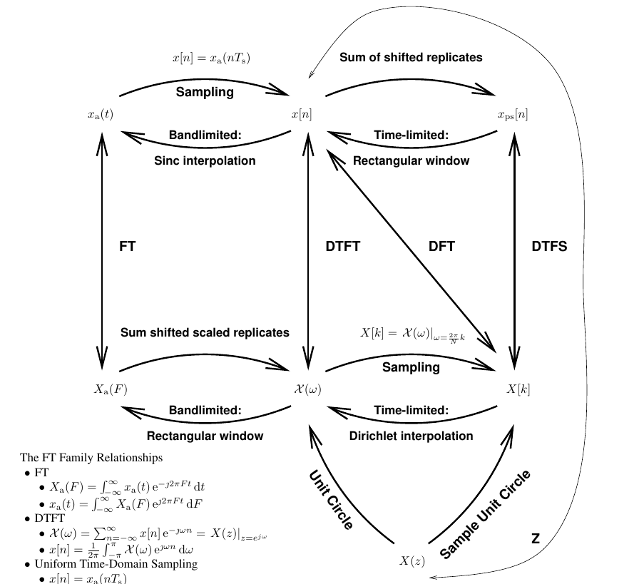
I found that Professor Jeffery Fessler’s note gives a clear picture of relations of different transforms. In general, the DFT is a simpified way to transform sampled time-domain sequences to sampled frequency-domain sequences.
Definition
For a sequence of $N$ complex numbers ${{f[n]}}_{n=0}^{N-1}$, the discrete Fourier Transform transforms the sequence into another sequence of complex numbers ${{\hat{f}[m]}}_{m=0}^{N-1}$:
\[\begin{equation} \hat{f}[m] = \sum_{n=0}^{N-1} f[n] e^{-i 2\pi k \frac{n}{N}} \end{equation}\]The inverse discrete Fourier transform is given by:
\[\begin{equation} f[n] = \frac{1}{N} \sum_{m=0}^{N-1} \hat{f}[m] e^{i 2\pi n \frac{m}{N}} \end{equation}\]Connection to the DTFT and DTFS
The DFT can be motivated by the sampling of the DTFT. Consider sampling the DTFT with $\Delta{k}$ sampling interval such that one period was sampled with exactly $N$ points ($N \Delta{k} = 1/\Delta{x}$):
\[\begin{equation} \begin{split} \hat{f}_{dtft}[m] &= \hat{f}_{dtft}(m\Delta{k})\\ &= \sum_{n=-\infty}^{\infty} f[n] e^{-i2\pi n\Delta{x} m\Delta{k}}\\ &= \sum_{n=-\infty}^{\infty} f[n] e^{-i2\pi \frac{nm}{N}} \end{split} \end{equation}\]Let’s break $f[n]$ into $N$-length segments such as $f[0] … f[N-1]$, $f[N] … f[2N-1]$, let $n=l-jN$ where $l \in [0, N-1]$ and $j \in [-\infty, \infty]$. Then $\hat{f}_{dtft}[m]$ can be redefined with $ N $-point periodic superposition:
\[\begin{equation} \begin{split} f_{ps}[l] = \sum_{j=-\infty}^{\infty} f[l-jN] \end{split} \end{equation}\] \[\begin{equation} \begin{split} \hat{f}_{dtft}[m] &= \sum_{n=-\infty}^{\infty} f[n] e^{-i2\pi \frac{nm}{N}}\\ &= \sum_{j=-\infty}^{\infty} \sum_{l=0}^{N-1} f[l-jN] e^{-i2\pi (l-jN) \frac{m}{N}}\\ &= \sum_{j=-\infty}^{\infty} \sum_{l=0}^{N-1} f[l-jN] e^{-i2\pi l \frac{m}{N}}\\ &= \sum_{l=0}^{N-1} \left(\sum_{j=-\infty}^{\infty} f[l-jN]\right) e^{-i2\pi l \frac{m}{N}}\\ &= \sum_{l=0}^{N-1} f_{ps}[l] e^{-i2\pi l \frac{m}{N}} \end{split} \end{equation}\]Obviously, $f_{ps}[l]$ is a $N$-periodic sequence. Since $f_{ps}[l]$ is $N$-periodic, it can be represented with the DTFS:
\[\begin{equation} \begin{split} c_m &= \sum_{l=0}^{N-1} f_{ps}[l] e^{-i 2\pi \frac{lm}{N}}\\ f_{ps}[l] &= \frac{1}{N} \sum_{m=0}^{N-1} c_m e^{i 2\pi \frac{ml}{N}} \end{split} \end{equation}\]Comparing the DTFS coefficients and the above DTFT samples, we see that:
\[\begin{equation} \begin{split} c_m &= \hat{f}_{dtft}[m] \end{split} \end{equation}\]Thus, we can recover the periodic sequence $f_{ps}[l]$ from those DTFT samples with the inverse DTFS:
\[\begin{equation} \begin{split} f_{ps}[l] &= \frac{1}{N} \sum_{m=0}^{N-1} \hat{f}_{dtft}[m] e^{i 2\pi \frac{ml}{N}} \end{split} \end{equation}\]However, this recovery does not ensure that we can recover the original sequence $f[n]$ with those DTFT samples. $f_{ps}[l]$ is a sum of shifted replicates of $f[n]$. Thus there is no perfect reconstruction for non time-limited sequences since time-domain replicates overlap and aliasing occurs.
There is a special case where time-domain replicates do not overlap. Considering a time-limited sequence $f[n]$ with duration $L$ which it has nonzero values only in the interval $0,…, L-1$. If $N \ge L$, then there is no overlap in the replicates. The original sequence $f[n]$ can be recovered from $f_{ps}[l]$:
\[\begin{equation} f[n] = \begin{cases} f_{ps}[n] & n \in [0, L-1)\\ 0 & \text{otherwise} \end{cases} \end{equation}\]In fact, if $f[n]$ is time-limited, the DTFT samples simplifies to a limited summation:
\[\begin{equation} \begin{split} \hat{f}[m] &= \hat{f}_{dtft}[m]\\ &= \sum_{n=0}^{L-1} f[n] e^{-i2\pi n \frac{m}{M}}\\ &= \sum_{n=0}^{N-1} f[n] e^{-i2\pi n \frac{m}{M}} \end{split} \end{equation}\]where $f[n]=0$ for $n \ge L$ and the above formula is called DFT and $f[n]$ can be recovered from the inverse DFT formula:
\[\begin{equation} \begin{split} f[n] = \begin{cases} \frac{1}{N} \sum_{m=0}^{N-1} \hat{f}[m] e^{i 2\pi \frac{mn}{N}} & n=0, ..., N-1\\ 0 & \text{otherwise} \end{cases} \end{split} \end{equation}\]