Total Variation Denoising Problem

Total variation (TV) denoising, also known as TV regularization or TV filtering, is a powerful technique widely used in various fields, including medical imaging, computer vision, etc. It removes noises while preserving most important structural features. The first image of black hole, captured by Event Horizon Telescope (EHT), was processed and revealed with this technique in 2019. The concept was proposed in 1992 by Rudin, Osher and Fatemi, known as the ROF model which is a continuous form of TV denoising problem.

What is Total Variation

The term, total variation, refers to a mathematical concept that is a little hard to understand for me. Nonrigorously, the TV of a function $u(x)$ is the integral of its derivative magnitude within its bouned domain $\Omega$:

$$\begin{equation} \begin{split} \|u\|_{TV} = \int_{\Omega} |\nabla u(x)| dx \end{split} \end{equation}$$

For practical use, a discretized version is more favorable. There are two common discretized TVs in literatures, the isotropic and anisotropic TVs. Suppose that $u(\mathcal{X})$ is a function of an order-$N$ tensor grid $\mathcal{X} \in \mathbb{R}^{I_1 \times I_2 \times \cdots I_N}$, the isotropic TV is defined as:

$$\begin{equation} \begin{split} \|u\|_{TV} = \sum_{i_1} \sum_{i_2} \cdots \sum_{i_N} \sqrt{\left(\nabla_{I_1} u \right)_{i_1 i_2 \cdots i_N}^2 + \cdots + \left(\nabla_{I_N} u \right)_{i_1 i_2 \cdots i_N}^2} \end{split} \end{equation}$$

where $\nabla_{I_k} u$ is the derivatives along the $I_k$ dimension. The isotropic TV is invariant to rotation of the domain that is if you rotate the image arbitrarily, the isotropic TV would not change.

The anisotropic TV is defined as:

$$\begin{equation} \begin{split} \|u\|_{TV} = \sum_{i_1} \sum_{i_2} \cdots \sum_{i_N} |\left(\nabla_{I_1} u \right)_{i_1 i_2 \cdots i_N}| + \cdots + |\left(\nabla_{I_N} u \right)_{i_1 i_2 \cdots i_N}| \end{split} \end{equation}$$

which is not rotation invariant. There is no difference between the isotropic and anisotropic TVs for 1D signals.

Discrete Derivatives

There are many ways to define derivatives for discretized signals. For better understanding, I will use a 1-d signal $u(x)$ (and its discrete form $u_i,i=0,1,2,\cdots,N-1$) as an example to illustrate all these ways. Let $\nabla_{x} u$ denote the derivatives of $u(x)$ in the x direction, $(\nabla_{x}^+ u)_i = u_{i+1} - u_i$ denote the forward difference, and $(\nabla_{x}^- u)_i = u_{i} - u_{i-1}$ denote the backward difference. A few definitions of derivatives are:

• one-sided difference, $(\nabla_{x}u)^2_{i} = (\nabla_{x}^+ u)^2_i$
• central difference, $(\nabla_{x}u)^2_{i} = (((\nabla_{x}^+ u)_i + (\nabla_{x}^- u)_i)/2)^2$
• geometric average, $(\nabla_{x}u)^2_{i} = ((\nabla_{x}^+ u)^2_i + (\nabla_{x}^- u)^2_i)/2$
• minmod difference, $(\nabla_{x}u)^2_{i} = m((\nabla_{x}^+ u)_i, (\nabla_{x}^- u)_i)$, where $m(a,b)=\left(\frac{sign(a) + sign(b)}{2}\right)min(|a|, |b|)$
• upwind discretization, $(\nabla_{x}u)^2_{i} = (max((\nabla_{x}^+ u)_i, 0)^2+max((\nabla_{x}^- u)_i, 0)^2)/2$

The one-sided difference (or forward difference) may be the most common way to discretize the derivatives but it’s not symmetric. Although the central difference is symmetric, it is not able to reveal thin and small structures (considering a single point with one and others are zero, the central difference at this point would be zero which is counter-intuitive). The geometric average, minmod difference and upwind discretization are both symmectic and being able to reveal thin structures at the cost of nonlinearity. I will use one-sided difference in the following content.

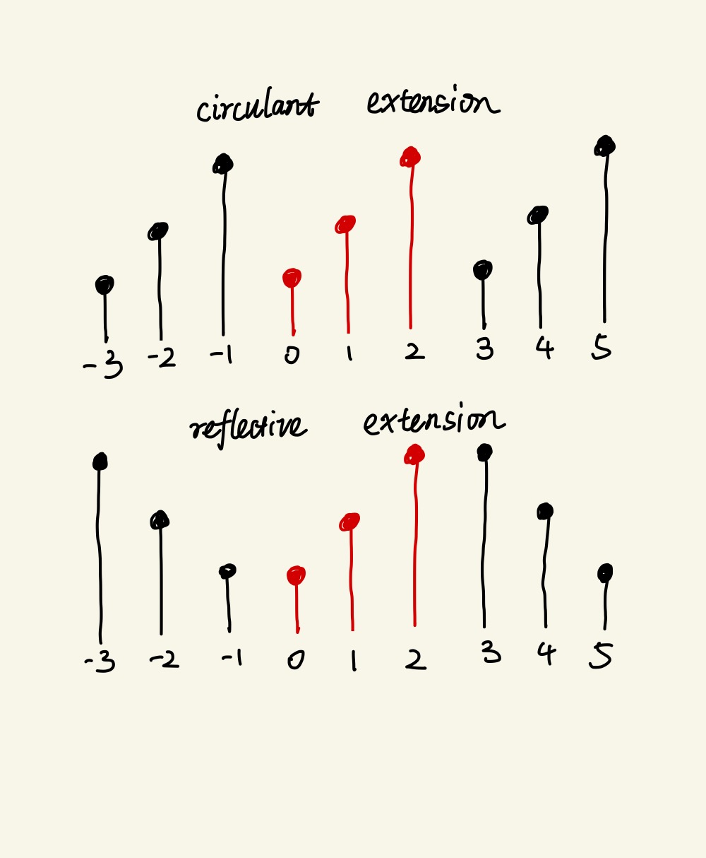
Since we are dealing with finite signals, special handling is needed on the boundaries. I have seen two common ways to do that in literatures. One is reflective extension and the other is circulant extension. The reflective extention assumes that the signals extend in a reflective way and the circulant extension assumes that the signals extend in a circulant way.

For the reflective extension, the matricized differential operator and its adjoint operator are:

$$\begin{equation} \begin{split} \mathbf{D} &= \begin{bmatrix} -1&1&&&\\ &-1&1&&\\ & &\ddots&\ddots&\\ & & &-1&1\\ &&&&0 \end{bmatrix}\\ \mathbf{D}^{\ast} &= - \begin{bmatrix} 1&&&&\\ -1&1&&&\\ &\ddots&\ddots&&\\ & &-1&1&\\ &&&-1&0 \end{bmatrix} = \mathbf{D}^T\\ \end{split} \end{equation}$$

For the circulant extension, the matricized differential operator and its adjoint operator are:

$$\begin{equation} \begin{split} \mathbf{D} &= \begin{bmatrix} -1&1&&&\\ &-1&1&&\\ & &\ddots&\ddots&\\ & & &-1&1\\ 1&&&&-1 \end{bmatrix}\\ \mathbf{D}^{\ast} &= - \begin{bmatrix} 1&&&&-1\\ -1&1&&&\\ &\ddots&\ddots&&\\ & &-1&1&\\ &&&-1&1 \end{bmatrix} = \mathbf{D}^T\\ \end{split} \end{equation}$$

As we’ve seen, the adjoint operators of differential operators are the negative backward differences. In practice, we don’t need to construct explicit matrices for those operators as long as we know how to perform the corresponding operations.

Total Variation Denoising

A general TV denoising problem minimizes the following objective function:

$$\begin{equation} \begin{split} \argmin_{u} \|u\|_{TV} + \frac{\lambda}{2} \|A(u) - v\|^2 \end{split} \end{equation}$$

where $u, v$ are functions of a given tensor grid $\mathcal{X}$, $A$ is a linear operator, and $\lambda$ controls how much smoothing is performed.

1D TV

Let’s make Equation (6) more concise for the 1D case:

$$\begin{equation} \begin{split} \argmin_{\mathbf{u} \in \mathbb{R}^N} \|\mathbf{D} \mathbf{u} \|_1 + \frac{\lambda}{2} \|\mathbf{A} \mathbf{u} - \mathbf{v}\|_2^2 \end{split} \end{equation}$$

where $\mathbf{A} \in \mathbb{R}^{M \times N}$ and $\mathbf{D}$ is the differential operator defined above.

Iterative Clipping

The iterative clipping method solves the 1D TV denoising problem by solving its dual form.

A useful fact is that the absolute value $|x|$ can be written as an optimization problem and the $l_1$ norm likewisely$:

$$\begin{equation} \begin{split} |x| &= \max_{|z| \le 1} zx \\ \|\mathbf{x}\|_1 &= \max_{|\mathbf{z}| \le 1} \mathbf{z}^T\mathbf{x} \end{split} \end{equation}$$

where $|\mathbf{z}| \le 1$ denotes each element of $\mathbf{z}$ is less than or equals to 1.

Let $F(\mathbf{u}) = \|\mathbf{D} \mathbf{u} \|_1 + \frac{\lambda}{2} \|\mathbf{A} \mathbf{u} - \mathbf{v}\|_2^2$, the objective function can be written as:

$$\begin{equation} \begin{split} F(\mathbf{u}) &= \max_{|\mathbf{z}| \le 1} \mathbf{z}^T\mathbf{D} \mathbf{u} + \frac{\lambda}{2} \|\mathbf{A} \mathbf{u} - \mathbf{v}\|_2^2\\ \end{split} \end{equation}$$

thus the Equation (7) can be written as:

$$\begin{equation} \begin{split} \arg &\min_{\mathbf{u}} \max_{|\mathbf{z}| \le 1} \mathbf{z}^T\mathbf{D} \mathbf{u} + \frac{\lambda}{2}\|\mathbf{A} \mathbf{u} - \mathbf{v}\|_2^2\\ \end{split} \end{equation}$$

The minmax theorem is that if the function $f(x, y)$ is concave in x and convex in y, then the following equlity holds:

$$\begin{equation} \begin{split} \max_{x} \min_{y} f(x, y) = \min_{y} \max_{x} f(x, y) \end{split} \end{equation}$$

then we can change the order of minmax in Equation (10):

$$\begin{equation} \begin{split} \arg \max_{|\mathbf{z}| \le 1} \min_{\mathbf{u}} \mathbf{z}^T\mathbf{D} \mathbf{u} + \frac{\lambda}{2}\|\mathbf{A} \mathbf{u} - \mathbf{v}\|_2^2\\ \end{split} \end{equation}$$

which is a dual form of the original problem.

The solution of the inner minimization problem is:

$$\begin{equation} \begin{split} \mathbf{u}_{k+1} &= \left(\mathbf{A}^T\mathbf{A}\right)^{\dag}\left(\mathbf{A}^T\mathbf{v} - \frac{1}{\lambda}\mathbf{D}^T\mathbf{z}_k\right) \end{split} \end{equation}$$

Substituting Equation (13) back into Equation (12) gives:

$$\begin{equation} \begin{split} \arg \min_{|\mathbf{z}| \le 1} \mathbf{z}^T\mathbf{D}\left(\mathbf{A}^T\mathbf{A}\right)^{\dag}\mathbf{D}^T\mathbf{z} - 2\lambda \left(\mathbf{D}\mathbf{A}^{\dag}\mathbf{v}\right)^T\mathbf{z} \end{split} \end{equation}$$

There are many ways to solve this quadratic form, one is by the majorization-minimization (MM) method. Given a function $F(x)$, the MM method chooses an auxiliary function $G_k(x)$ such that $G_k(x) \ge F(x),\ G_k(x_k) = F(x_k)$, then solves $x_{k+1}=\argmin_{x} G_k(x)$. The sequence $x_k$ converges to the minimizer of $F(x)$ when $F(x)$ is convex.

We construct such a function $G_k(\mathbf{z})$ by adding $\left(\mathbf{z} - \mathbf{z}_k\right)^T\left(\alpha\mathbf{I} - \mathbf{D}\left(\mathbf{A}^T\mathbf{A}\right)^{\dag}\mathbf{D}^T\right)(\mathbf{z} - \mathbf{z}_k)$ to Equation (14):

$$\begin{equation} \begin{split} G_k(\mathbf{z}) &= \mathbf{z}^T\mathbf{D}\left(\mathbf{A}^T\mathbf{A}\right)^{\dag}\mathbf{D}^T\mathbf{z} - 2\lambda \left(\mathbf{D}\mathbf{A}^{\dag}\mathbf{v}\right)^T\mathbf{z}\\ &+\left(\mathbf{z} - \mathbf{z}_k\right)^T\left(\alpha\mathbf{I} - \mathbf{D}\left(\mathbf{A}^T\mathbf{A}\right)^{\dag}\mathbf{D}^T\right)(\mathbf{z} - \mathbf{z}_k) \end{split} \end{equation}$$

where $\alpha \ge \lambda_0(\mathbf{D}\left(\mathbf{A}^T\mathbf{A}\right)^{\dag}\mathbf{D}^T)$ (the max eigenvalue) such that this term is always positive-semidefinite.

Simplifing Equation (15) gives:

$$\begin{equation} \begin{split} \arg \min_{|\mathbf{z}| \le 1} \mathbf{z}^T\mathbf{z} - 2\left(\mathbf{z}_k + \frac{\lambda}{\alpha} \mathbf{D} \mathbf{u}_{k+1}\right)^T\mathbf{z} \end{split} \end{equation}$$

which is a separable quadratic optimization problem for each element of $\mathbf{z}$. The solution of the above problem is:

$$\begin{equation} \begin{split} \mathbf{z}_{k+1} &= clip(\mathbf{z}_k + \frac{\lambda}{\alpha} \mathbf{D}\mathbf{u}_{k+1}, 1) \end{split} \end{equation}$$

where $clip(x, T)$ is a function clippling the input $x$:

$$\begin{equation} \begin{split} clip(x, T) = \begin{cases} |x| & |x| \le T\\ sign(x)T & otherwise\\ \end{cases} \end{split} \end{equation}$$

We can scale $\mathbf{z}$ by $\frac{1}{\lambda}$, then the iterative clipping method iterates as the following:

$$\begin{equation} \begin{split} \mathbf{u}_{k+1} &= \left(\mathbf{A}^T\mathbf{A}\right)^{\dag}\left(\mathbf{A}^T\mathbf{v} - \mathbf{D}^T\mathbf{z}_k\right)\\ \mathbf{z}_{k+1} &= clip(\mathbf{z}_k + \frac{1}{\alpha} \mathbf{D}\mathbf{u}_{k+1}, \frac{1}{\lambda})\\ \end{split} \end{equation}$$

where $\alpha \ge \lambda_0(\mathbf{D}\left(\mathbf{A}^T\mathbf{A}\right)^{\dag}\mathbf{D}^T)$.

It turns out that the method can be accelerated with a smaller $\alpha$ value by contraction mapping principle (basically, it means that there is a fixed point such that $f(x)=x$). To make $\mathbf{z}_k + \frac{1}{\alpha} \mathbf{D}\mathbf{u}_{k+1}$ a contraction function, we need to make sure $\mathbf{I} - \frac{1}{\alpha}\mathbf{D}\left(\mathbf{A}^T\mathbf{A}\right)^{\dag}\mathbf{D}^T$ is a contraction function. It suggests that $\alpha \gt \lambda_0(\mathbf{D}\left(\mathbf{A}^T\mathbf{A}\right)^{\dag}\mathbf{D}^T)/2$, which halves the original value.

If $\mathbf{A} = \mathbf{I}$, then Equation (7) becomes the naive TV denoising problem. It turns out that $\lambda_0(\mathbf{D}\mathbf{D}^T)$ is less than 4 regardless of $N$ for both definitions in Equation (4) and (5), thus $\alpha = 2.3$ is an appropriate option for $\mathbf{A} = \mathbf{I}$.

Majorization Minimization

We could also derive an algorithm with the MM method directly. Given $F(x) = |x|$ for scalar $x$, then $G(x) = \frac{1}{2|x_k|}x^2 + \frac{1}{2}|x_k|$ such that $G(x) \ge F(x)$ and $G(x_k) = F(x_k)$. For the $l_1$ norm, $G(\mathbf{x})$ is:

$$\begin{equation} \begin{split} G(\mathbf{x}) &= \frac{1}{2} \mathbf{x}^T\mathbf{\Lambda}_k^{-1}\mathbf{x} + \frac{1}{2}\|\mathbf{x}_k\|_1 \end{split} \end{equation}$$

where $\mathbf{\Lambda}_k=diag(|\mathbf{x}_k|)$.

A majorizer of the TV cost function in Equation (7) is:

$$\begin{equation} \begin{split} \argmin_{\mathbf{u}} \frac{1}{2} \mathbf{u}^T\mathbf{\Lambda}_k^{-1}\mathbf{u} + \frac{1}{2}\|\mathbf{u}_k\|_1 + \frac{\lambda}{2} \|\mathbf{A} \mathbf{u} - \mathbf{v}\|_2^2 \end{split} \end{equation}$$

Since the $l_1$ term above is now a constant, it’s easier to derive an explicit solution:

$$\begin{equation} \begin{split} \mathbf{u}_{k+1} = \left(\mathbf{A}^T\mathbf{A} + \frac{1}{\lambda} \mathbf{D}^T\mathbf{\Lambda}_k^{-1}\mathbf{D}\right)^{\dag} \mathbf{A}^T \mathbf{v} \end{split} \end{equation}$$

A problem with this iteration form is that as the iterations progress, some values of $\mathbf{\Lambda}_k$ will go to zero, causing division-by-zero errors. This issue can be solved with the matrix inverse lemma:

$$\begin{equation} \begin{split} \mathbf{u}_{k+1} &= \left(\left(\mathbf{A}^T\mathbf{A}\right)^{\dag} - \left(\mathbf{A}^T\mathbf{A}\right)^{\dag} \mathbf{D}^T \left(\lambda \mathbf{\Lambda}_k + \mathbf{D} \left(\mathbf{A}^T\mathbf{A}\right)^{\dag} \mathbf{D}^T \right)^{\dag} \mathbf{D} \left(\mathbf{A}^T\mathbf{A}\right)^{\dag} \right) \mathbf{A}^T \mathbf{v}\\ &= \mathbf{A}^{\dag}\mathbf{v} - \left(\mathbf{A}^T\mathbf{A}\right)^{\dag}\mathbf{D}^T \left(\lambda \mathbf{\Lambda}_k + \mathbf{D} \left(\mathbf{A}^T\mathbf{A}\right)^{\dag} \mathbf{D}^T \right)^{\dag} \mathbf{D} \mathbf{A}^{\dag} \mathbf{v} \end{split} \end{equation}$$

The complexity of the algorithm would depends on how quick to solve linear equations $\left(\lambda \mathbf{\Lambda}_k + \mathbf{D} \left(\mathbf{A}^T\mathbf{A}\right) \mathbf{D}^T\right) \mathbf{x} = \mathbf{D} \mathbf{A}^{\dag} \mathbf{v}$. If $\mathbf{A} = \mathbf{I}$, then $\lambda \mathbf{\Lambda}_k + \mathbf{D}\mathbf{D}^T$ is a banded matrix which can be solved fastly.

The matrix inverse lemma is:

$$\begin{equation} \begin{split} (\mathbf{A} + \mathbf{B}\mathbf{C}\mathbf{D})^{-1} = \mathbf{A}^{-1} - \mathbf{A}^{-1}\mathbf{B}(\mathbf{C}^{-1} + \mathbf{D}\mathbf{A}^{-1}\mathbf{B})^{-1}\mathbf{D}\mathbf{A}^{-1} \end{split} \end{equation}$$

Split Bregman

I wrote more about the split Bregman method in another post. Here I briefly give the method. To solve the following problem:

$$\begin{equation} \begin{split} \argmin_{\mathbf{x}}\ \|F(\mathbf{x})\|_1 + \lambda G(\mathbf{x}) \end{split} \end{equation}$$

where $F(\mathbf{x})$ and $G(\mathbf{x})$ are both convex and differentiable. $F(\mathbf{x})$ is also linear.

By setting $\mathbf{d} = F(\mathbf{x})$,the split Bregman method has the following iterations:

$$\begin{equation} \begin{split} \mathbf{x}_{k+1} &= \argmin_{\mathbf{x}}\ \lambda G(\mathbf{x}) + \frac{\mu}{2}\|F(\mathbf{x}) - \mathbf{d}_k - \mathbf{b}_k \|_2^2\\ \mathbf{d}_{k+1} &= \argmin_{\mathbf{d}}\ \|\mathbf{d}\|_1 + \frac{\mu}{2}\|F(\mathbf{x}_{k+1}) - \mathbf{d} - \mathbf{b}_k \|_2^2\\ \mathbf{b}_{k+1} &= \mathbf{b}_k - F(\mathbf{x}_{k+1}) + \mathbf{d}_{k+1} \end{split} \end{equation}$$

Now back to our 1D TV denoising problem in Equation (7), let $\mathbf{d}=\mathbf{D}\mathbf{u}$ and apply the above split Bregman method, we have:

$$\begin{equation} \begin{split} \mathbf{u}_{k+1} &= \argmin_{\mathbf{u}}\ \frac{\lambda}{2} \|\mathbf{A} \mathbf{u} - \mathbf{v}\|_2^2 + \frac{\mu}{2}\|\mathbf{D}\mathbf{u} - \mathbf{d}_k - \mathbf{b}_k \|_2^2\\ \mathbf{d}_{k+1} &= \argmin_{\mathbf{d}}\ \|\mathbf{d}\|_1 + \frac{\mu}{2}\|\mathbf{D}\mathbf{u}_{k+1} - \mathbf{d} - \mathbf{b}_k \|_2^2\\ \mathbf{b}_{k+1} &= \mathbf{b}_k - \mathbf{D}\mathbf{u}_{k+1} + \mathbf{d}_{k+1} \end{split} \end{equation}$$

The first subproblem can be solved by setting the derivative to zero and solving equations:

$$\begin{equation} \begin{split} \left(\lambda \mathbf{A}^T\mathbf{A} + \mu \mathbf{D}^T\mathbf{D}\right)\mathbf{u}_{k+1} = \lambda \mathbf{A}^T\mathbf{v} + \mu \mathbf{D}^T(\mathbf{d}_k + \mathbf{b}_k) \end{split} \end{equation}$$

and the second subproblem has an explicit solution:

$$\begin{equation} \begin{split} \mathbf{d}_{k+1} = S_{1/\mu}[\mathbf{D}\mathbf{u}_{k+1} + \mathbf{b}_k] \end{split} \end{equation}$$

where $S_t(\cdot)$ is the soft-thresholding operator introduced in this post.

ADMM

Alternating Direction Method of Multipliers (ADMM) is definitely the most widely used algorithm to solve L1-regularized problems, especially in MRI. For a separable problem with equality constraints:

$$\begin{equation} \begin{split} \argmin_{\mathbf{x}, \mathbf{y}}&\ F(\mathbf{x}) + G(\mathbf{y})\\ &s.t.\ \mathbf{A}\mathbf{x} + \mathbf{B}\mathbf{y} = \mathbf{c} \end{split} \end{equation}$$

with its augmented Lagrangian form $L_{\rho}(\mathbf{x}, \mathbf{y}, \mathbf{v})= F(\mathbf{x}) + G(\mathbf{y}) + \mathbf{v}^T(\mathbf{A}\mathbf{x} + \mathbf{B}\mathbf{y} - \mathbf{c}) + \frac{\rho}{2} \|\mathbf{A}\mathbf{x} + \mathbf{B}\mathbf{y} - \mathbf{c}\|_2^2$, the ADMM iteration is like:

$$\begin{equation} \begin{split} \mathbf{x}_{k+1} &= \argmin_{\mathbf{x}} L_{\rho}(\mathbf{x}, \mathbf{y}_k, \mathbf{v}_k)\\ \mathbf{y}_{k+1} &= \argmin_{\mathbf{y}} L_{\rho}(\mathbf{x}_{k+1}, \mathbf{y}, \mathbf{v}_k)\\ \mathbf{v}_{k+1} &= \mathbf{v}_k + \rho (\mathbf{A}\mathbf{x}_{k+1} + \mathbf{B}\mathbf{y}_{k+1} - \mathbf{c}) \end{split} \end{equation}$$

Let $\mathbf{d}=\mathbf{D}\mathbf{u}$ and we would find that our 1D TV denoising problem falls within the ADMM form, thus we have the following iteration:

$$\begin{equation} \begin{split} \mathbf{u}_{k+1} &= \argmin_{\mathbf{u}} L_{\rho}(\mathbf{u}, \mathbf{d}_k, \mathbf{y}_k)\\ \mathbf{d}_{k+1} &= \argmin_{\mathbf{d}} L_{\rho}(\mathbf{u}_{k+1}, \mathbf{d}, \mathbf{y}_k)\\ \mathbf{y}_{k+1} &= \mathbf{y}_k + \rho (\mathbf{D}\mathbf{y}_{k+1} -\mathbf{d}_{k+1}) \end{split} \end{equation}$$

where $L_{\rho}(\mathbf{u}, \mathbf{d}_k, \mathbf{y}_k)$ is:

$$\begin{equation} \begin{split} L_{\rho}(\mathbf{u}, \mathbf{d}, \mathbf{y}) &= \|\mathbf{d}\|_1 + \frac{\lambda}{2} \|\mathbf{A}\mathbf{u} - \mathbf{v}\|_2^2 \\&+ \mathbf{y}^T(\mathbf{D}\mathbf{u} - \mathbf{d}) + \frac{\rho}{2} \|\mathbf{D}\mathbf{u} - \mathbf{d} \|_2^2 \end{split} \end{equation}$$

The first subproblem can be solved by setting the derivative to zero:

$$\begin{equation} \begin{split} (\lambda\mathbf{A}^T\mathbf{A} + \rho \mathbf{D}^T\mathbf{D})\mathbf{u}_{k+1} &= \lambda\mathbf{A}^T\mathbf{v} + \mathbf{D}^T(\rho \mathbf{d}_k - \mathbf{y}_k) \end{split} \end{equation}$$

and the solution of the second subproblem is:

$$\begin{equation} \begin{split} \mathbf{d}_{k+1} = S_{1/\rho}[\mathbf{D}\mathbf{u}_{k+1} + \frac{1}{\rho} \mathbf{y}_k] \end{split} \end{equation}$$

2D TV

As we’ve already known in previous section, there are two types of TVs for high-dimensional data. Equation (6) for the 2D case with the isotrophic TV is like:

$$\begin{equation} \begin{split} \argmin_{\mathbf{u} \in \mathbb{R}^{MN}} \sum_{i} \sum_{j} \sqrt{\left(\nabla_{I} \mathbf{u} \right)_{i,j}^2 + \left(\nabla_{J} \mathbf{u} \right)_{i,j}^2} + \frac{\lambda}{2} \|A\mathbf{u} - \mathbf{v}\|_2^2 \end{split} \end{equation}$$

where $A(\cdot)\colon \mathbb{R}^{MN} \longmapsto \mathbb{R}^{K}$ is a linear function acts on vectorized matrix $\mathbf{u}$ and $\mathbf{v} \in \mathbb{R}^{K}$ is measured signals. With the anisotrophic TV, Equation (6) is going to be like:

$$\begin{equation} \begin{split} \argmin_{\mathbf{u} \in \mathbb{R}^{MN}} \sum_{i} \sum_{j} \left(|\nabla_{I} \mathbf{u} |_{i,j} + |\nabla_{J} \mathbf{u} |_{i,j}\right) + \frac{\lambda}{2} \|A\mathbf{u} - \mathbf{v}\|_2^2 \end{split} \end{equation}$$

Note that the differential operator $\nabla_{I}$ acts on vectorized matrices and returns two-dimensional matrices. It’s easier to derive gradients with vectorized matrices rather than matrices themselves. Keep in mind that We don’t actually construct explit differential matrices for $\nabla_{I}$ and its adjoint. For example, we could reshape vectors into matrices and perform forward differential operations along the corresponding dimension. For $\nabla_{I}^*$, which acts on matrices and returns vectorized matrices, we could perform backward differential operations along the corresponding dimension, then negative all elements, finally reshape matrices into vectors.

Split Bregman

To apply the split Bregman method to Equation (36), we need to simplify the TV term by setting $\mathbf{D}_I = \nabla_{I} \mathbf{u}$ and $\mathbf{D}_J = \nabla_{J} \mathbf{u}$:

$$\begin{equation} \begin{split} \argmin_{\mathbf{u} \in \mathbb{R}^{MN}} &\ \sum_{i} \sum_{j} \sqrt{\left(\mathbf{D}_{I} \right)_{i,j}^2 + \left(\mathbf{D}_{J} \right)_{i,j}^2} + \frac{\lambda}{2} \|\mathbf{A}\mathbf{u} - \mathbf{v}\|_2^2\\ s.t &\ \mathbf{D}_I = \nabla_{I} \mathbf{u}\\ &\ \mathbf{D}_J = \nabla_{J} \mathbf{u} \end{split} \end{equation}$$

The iteration is like:

$$\begin{equation} \begin{split} \mathbf{u}_{k+1} &= \argmin_{\mathbf{u}} \frac{\lambda}{2} \|A\mathbf{u} - \mathbf{v}\|_2^2 + \frac{\mu}{2} \|\begin{bmatrix}\mathbf{D}_{I,k}\\ \mathbf{D}_{J,k}\end{bmatrix} - \begin{bmatrix}\nabla_I \mathbf{u} \\ \nabla_J \mathbf{u}\end{bmatrix} - \begin{bmatrix}\mathbf{B}_{I,k} \\ \mathbf{B}_{J,k} \end{bmatrix}\|_F^2\\ \mathbf{D}_{I, k+1}, \mathbf{D}_{J, k+1} &= \argmin_{\mathbf{D}_{I}, \mathbf{D}_{J}} \sum_{i} \sum_{j} \sqrt{\left(\mathbf{D}_{I} \right)_{i,j}^2 + \left(\mathbf{D}_{J} \right)_{i,j}^2} + \frac{\mu}{2} \|\begin{bmatrix}\mathbf{D}_{I}\\ \mathbf{D}_{J}\end{bmatrix} - \begin{bmatrix}\nabla_I \mathbf{u}_{k+1} \\ \nabla_J \mathbf{u}_{k+1}\end{bmatrix} - \begin{bmatrix}\mathbf{B}_{I,k} \\ \mathbf{B}_{J,k} \end{bmatrix}\|_F^2\\ \begin{bmatrix}\mathbf{B}_{I,k+1} \\ \mathbf{B}_{J,k+1} \end{bmatrix} &= \begin{bmatrix}\mathbf{B}_{I,k} \\ \mathbf{B}_{J,k} \end{bmatrix} + \begin{bmatrix}\nabla_I \mathbf{u}_{k+1} \\ \nabla_J \mathbf{u}_{k+1}\end{bmatrix} - \begin{bmatrix}\mathbf{D}_{I,k+1}\\ \mathbf{D}_{J,k+1}\end{bmatrix} \end{split} \end{equation}$$

The first subproblem can be solved with setting its derivative to zero:

$$\begin{equation} \begin{split} \left(\lambda \mathbf{A}^*\mathbf{A} + \mu\left( \nabla_I^*\nabla_I + \nabla_J^*\nabla_J\right)\right)\mathbf{u} &= \lambda\mathbf{A}^*\mathbf{v} + \mu \left(\nabla_I^*\mathbf{Z}_{I,k} + \nabla_J^*\mathbf{Z}_{J,k}\right)\\ \mathbf{Z}_{I,k} &= \mathbf{D}_{I,k} - \mathbf{B}_{I,k}\\ \mathbf{Z}_{J,k} &= \mathbf{D}_{J,k} - \mathbf{B}_{J,k}\\ \end{split} \end{equation}$$

The second subproblem can be solved by letting $\mathbf{w}_{i,j} = \begin{bmatrix}(\mathbf{D}_{I})_{i,j}\\ (\mathbf{D}_{J})_{i,j}\end{bmatrix}$, then the subproblem can be transformed into:

$$\begin{equation} \begin{split} \argmin_{all \mathbf{w}_{i,j}s} &\ \sum_{i} \sum_{j} \|\mathbf{w}_{i,j}\|_2 + \frac{\mu}{2} \sum_{i} \sum_{j} \|\mathbf{w}_{i,j} - \mathbf{y}_{i,j}\|_2^2\\ &\ \mathbf{y}_{i,j} = \begin{bmatrix} (\nabla_I \mathbf{u}_{k+1}-\mathbf{B}_{I,k})_{i,j} \\ (\nabla_J \mathbf{u}_{k+1}-\mathbf{B}_{J,k})_{i,j}\end{bmatrix} \end{split} \end{equation}$$

We should know that for the 2nd-norm proximal problem:

$$\begin{equation} \begin{split} \argmin_{\mathbf{x}} &\ \|\mathbf{x}\|_2 + \frac{1}{2t} \|\mathbf{x} - \mathbf{y}\|_2^2 \end{split} \end{equation}$$

it has an explict solution known as vectorial shrinkage:

$$\begin{equation} \begin{split} \mathbf{x}^* = S_t[\|\mathbf{y}\|_2] \frac{\mathbf{y}}{\|\mathbf{y}\|_2} \end{split} \end{equation}$$

The equation (41) is obviously separable for all $\mathbf{w}_{i,j}$s and each separable subproblem has the solution we list above:

$$\begin{equation} \begin{split} \mathbf{w}_{i,j}^* &= \begin{bmatrix}(\mathbf{D}_{I,k+1})_{i,j}\\ (\mathbf{D}_{J,k+1})_{i,j}\end{bmatrix}\\ &= S_{1/\mu}[\|\mathbf{y}_{i,j}\|_2] \frac{\mathbf{y}_{i,j}}{\|\mathbf{y}_{i,j}\|_2} \end{split} \end{equation}$$

To apply the split Bregman method to Equation (37) by letting $\mathbf{D}_I = \nabla_{I} \mathbf{u}$ and $\mathbf{D}_J = \nabla_{J} \mathbf{u}$, the only difference is the 2nd subproblem:

$$\begin{equation} \begin{split} \mathbf{D}_{I, k+1}, \mathbf{D}_{J, k+1} = \argmin_{\mathbf{D}_{I}, \mathbf{D}_{J}} &\|vec(\mathbf{D}_I)\|_1 + \|vec(\mathbf{D}_J)\|_1\\ &+ \frac{\mu}{2} \|vec(\mathbf{D}_I -\nabla_I\mathbf{u}_{k+1} - \mathbf{B}_{I,k}\|_2^2)\\ &+ \frac{\mu}{2} \|vec(\mathbf{D}_J -\nabla_J\mathbf{u}_{k+1} - \mathbf{B}_{J,k}\|_2^2) \end{split} \end{equation}$$

which can be solved with soft-thresholding:

$$\begin{equation} \begin{split} \mathbf{D}_{I, k+1} &= S_{1/\mu}[\nabla_I \mathbf{u}_{k+1} + \mathbf{B}_{I, k}]\\ \mathbf{D}_{J, k+1} &= S_{1/\mu}[\nabla_J \mathbf{u}_{k+1} + \mathbf{B}_{J, k}]\\ \end{split} \end{equation}$$

ADMM

To apply ADMM to equation (36) by letting $\mathbf{D}_I = \nabla_{I} \mathbf{u}$ and $\mathbf{D}_J = \nabla_{J} \mathbf{u}$, the augmented Lagrangian form is:

$$\begin{equation} \begin{split} L_{\rho}(\mathbf{u}, \mathbf{D}_I,\mathbf{D}_J, \mathbf{Y}_I, \mathbf{Y}_J) = &\sum_i\sum_j \sqrt{(\mathbf{D}_I)_{i,j}^2 + (\mathbf{D}_J)_{i,j}^2} + \frac{\lambda}{2} \|A\mathbf{u} - \mathbf{v}\|_2^2\\ &+ \frac{\rho}{2} \|\nabla_I\mathbf{u} - \mathbf{D}_{I,k} + \mathbf{Y}_{I,k}\|_F^2\\ &+ \frac{\rho}{2} \|\nabla_J\mathbf{u} - \mathbf{D}_{J,k} + \mathbf{Y}_{J,k}\|_F^2 \end{split} \end{equation}$$

The ADMM iteration is like:

$$\begin{equation} \begin{split} \mathbf{u}_{k+1} &= \argmin_{\mathbf{u}} \frac{\lambda}{2} \|A\mathbf{u} - \mathbf{v}\|_2^2 + \frac{\rho}{2} \|\nabla_I\mathbf{u} - \mathbf{D}_{I,k} + \mathbf{Y}_{I,k}\|_F^2 + \frac{\rho}{2} \|\nabla_J\mathbf{u} - \mathbf{D}_{J,k} + \mathbf{Y}_{J,k}\|_F^2\\ \mathbf{D}_{I,k+1}, \mathbf{D}_{J,k+1} &= \argmin_{\mathbf{D}_I, \mathbf{D}_J} \sum_i\sum_j \sqrt{(\mathbf{D}_I)_{i,j}^2 + (\mathbf{D}_J)_{i,j}^2} + \frac{\rho}{2} \|\nabla_I\mathbf{u}_{k+1} - \mathbf{D}_{I} + \mathbf{Y}_{I,k}\|_F^2 + \frac{\rho}{2} \|\nabla_J\mathbf{u}_{k+1} - \mathbf{D}_{J} + \mathbf{Y}_{J,k}\|_F^2\\ \mathbf{Y}_{I,k+1} &= \mathbf{Y}_{I,k} + (\nabla_I\mathbf{u}_{k+1} - \mathbf{D}_{I, k+1})\\ \mathbf{Y}_{J,k+1} &= \mathbf{Y}_{J,k} + (\nabla_J\mathbf{u}_{k+1} - \mathbf{D}_{J, k+1}) \end{split} \end{equation}$$

The solution of the first subproblem is:

$$\begin{equation} \begin{split} (\lambda \mathbf{A}^*\mathbf{A} + \rho (\nabla_I^*\nabla_I + \nabla_J^*\nabla_J))\mathbf{u} &= \lambda \mathbf{A}^*\mathbf{v} + \rho (\nabla_I^* \mathbf{Z}_{I,k} + \nabla_J^*\mathbf{Z}_{J,k})\\ \mathbf{Z}_{I,k} &= \mathbf{D}_{I,k} - \mathbf{Y}_{I,k}\\ \mathbf{Z}_{J,k} &= \mathbf{D}_{J,k} - \mathbf{Y}_{J,k} \end{split} \end{equation}$$

The second subproblem can be solved as the same process in split Bregman by letting $\mathbf{w}_{i,j} = \begin{bmatrix}(\mathbf{D}_{I})_{i,j}\\ (\mathbf{D}_{J})_{i,j}\end{bmatrix}$:

$$\begin{equation} \begin{split} \mathbf{w}_{i,j}^* &= \begin{bmatrix}(\mathbf{D}_{I,k+1})_{i,j}\\ (\mathbf{D}_{J,k+1})_{i,j}\end{bmatrix}\\ &= S_{1/\rho}[\|\mathbf{y}_{i,j}\|_2] \frac{\mathbf{y}_{i,j}}{\|\mathbf{y}_{i,j}\|_2}\\ \mathbf{y}_{i,j} &= \begin{bmatrix} (\nabla_I \mathbf{u}_{k+1}+\mathbf{Y}_{I,k})_{i,j} \\ (\nabla_J \mathbf{u}_{k+1}+\mathbf{Y}_{J,k})_{i,j}\end{bmatrix} \end{split} \end{equation}$$

The ADMM iteration to equation (37) is like:

$$\begin{equation} \begin{split} (\lambda \mathbf{A}^*\mathbf{A} + \rho (\nabla_I^*\nabla_I + \nabla_J^*\nabla_J))\mathbf{u} &= \lambda \mathbf{A}^*\mathbf{v} + \rho (\nabla_I^* \mathbf{Z}_{I,k} + \nabla_J^*\mathbf{Z}_{J,k})\\ \mathbf{Z}_{I,k} &= \mathbf{D}_{I,k} - \mathbf{Y}_{I,k}\\ \mathbf{Z}_{J,k} &= \mathbf{D}_{J,k} - \mathbf{Y}_{J,k}\\ \mathbf{D}_{I,k+1} &= S_{1/\rho}[\nabla_I\mathbf{u}_{k+1} + \mathbf{Y}_{I,k}]\\ \mathbf{D}_{J,k+1} &= S_{1/\rho}[\nabla_J\mathbf{u}_{k+1} + \mathbf{Y}_{J,k}]\\ \mathbf{Y}_{I,k+1} &= \mathbf{Y}_{I,k} + (\nabla_I\mathbf{u}_{k+1} - \mathbf{D}_{I, k+1})\\ \mathbf{Y}_{J,k+1} &= \mathbf{Y}_{J,k} + (\nabla_J\mathbf{u}_{k+1} - \mathbf{D}_{J, k+1}) \end{split} \end{equation}$$