Dive into ESPIRiT, from Theory to Practice 2
This post summarizes some practical implementation details for making ESPIRiT more efficient. Here are some notations I would use in the following discussions:
- $\mathbf{X} \in \mathbb{C}^{N_x \times N_y \times N_z \times N_c}$, a 3D kspace input with $N_c$ channels, $N=N_x N_y N_z N_c$
- $\mathbf{X}_{calib} \in \mathbb{C}^{M_x \times M_y \times M_z \times N_c}$, the calibration data of $\mathbf{X}$
- a kernel of size $K_x \times K_y \times K_z \times N_c$, $M = K_x K_y K_z$
- $\mathbf{V}_{\parallel} \in \mathbb{C^{MN_c \times N_k}}$, the row space vectors of calibration matrix $\mathbf{A}$, $N_k$ is the dimension of the row space
Problems of A Naive Algorithm
My previous post explores the mathematical theory behind ESPIRiT and derives the following steps to compute coil sensitives:
- Reshape $\mathbf{V}_{\parallel}$ to the shape $M \times N_c \times N_k$
- Center it and pad it to the full-grid size $N \times N_c \times N_k$
- Apply the inverse Fourier transform on the conjugated k-space kernels
- Extract $\mathbf{G}_n$ of shape $N_c \times N_k$ for each pixel $n$
- Compute eigenvectors of $M^{-1}N\mathbf{G}_n\mathbf{G}_n^H$
- Select the eigenvectors corresponding to the eigenvalues of 1, which represent the coil sensitivities at pixel $n$
- Repeat 4 to 6 until all pixels have been processed
One of problems from the above algorithm is that it allocates too much memory in practice. The calibration matrix $\mathbf{A}$, constructed from local patches of the calibration data, has shape $(M_x-K_x+1)(M_y-K_y+1)(M_z-K_z+1) \times K_x K_y K_z N_c$. Steps 1 to 3 produce a tensor of shape $N_x \times N_y \times N_z \times N_c \times N_k$. In practice, $K_x K_y K_z N_c$ can be up to a thousand, which can make this tensor tens of gigabytes in size. For example, a 3D volume of shape $256 \times 256 \times 256$ with $24$ channels would easily take up 37GB if $N_k = 100$.
Another problem origins from the separability characteristic of the algorithm. Note that steps 4 to 7 produce $N_c$ values for each pixel in parallel. It’s typically useful nowadays, as we can maximally take advantage of the parallel computing capabilities of modern hardware, such as GPUs. However, it also leads to the phase ambiguity problem in complex svd or eig. I have previously written a post about the sign ambiguity problem in real svd or eig, which is quite similar. In mathematics, you can add an arbitrary phase to both singular vectors (or eigenvectors) without breaking the constraints:
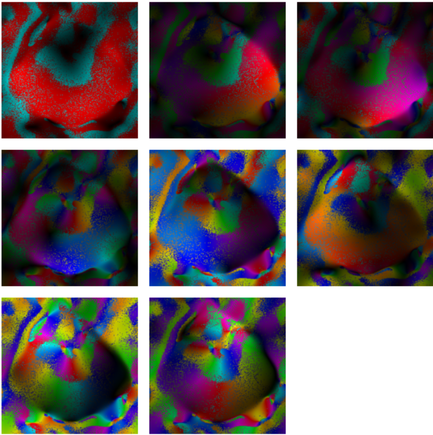
\[\begin{equation} \begin{split} \sigma \mathbf{u} e^{i\theta} (\mathbf{v} e^{i\theta})^H &= \sigma \mathbf{u} e^{i\theta} e^{-i\theta} \mathbf{v}^H\\ &= \sigma \mathbf{u}\mathbf{v}^H \end{split} \label{eq:1} \end{equation}\]In other words, each svd adds “random” phases to its singular vectors, so the phases of the coil sensitivies are not the true physical phases. To be clear, svd and eig are deterministic, as their underlying implementations implicitly choose a specific phase for the outputs, ensuring that you always get the same results for the same input. However, when considering a group of SVDs, the choosed phases can appear quite random relative to each other. The following figure shows eight coil sensitivies estimated by the naive algorithm. Each coil sensitivity appears an noisy phase distribution, yet this distribution is consistent across multiple maps.

The remaining problem is how to choose predefined parameters in the algorithm, such as the kernel size and null space threshold.
Simplify Steps 1 to 4
As we discussed earlier, the memory cost of $\mathbf{G}_n$ is usually high for 3D inputs. One way to reduce the cost is to compute $\mathbf{G}_n\mathbf{G}_n^H$ directly, resulting in a tensor of shape $N_x \times N_y \times N_z \times N_c \times N_c$. Since $N_c$ is generally much smaller than $N_k$, a considerable memory reduction can be expected.
As proved in the previous post, for each location $n$, coil sensitivies can be estimated by eigenvalue decomposition of the following matrix:
\[\begin{equation} \begin{split} M^{-1} \begin{bmatrix} \hat{\mathbf{K}}_{1,1}(n) & \cdots & \hat{\mathbf{K}}_{1,N_c}(n)\\ \vdots & \ddots & \vdots\\ \hat{\mathbf{K}}_{N_c,1}(n) & \cdots & \hat{\mathbf{K}}_{N_c,N_c}(n)\\ \end{bmatrix} \end{split} \end{equation}\]where
\[\begin{equation} \begin{split} \hat{\mathbf{K}}_{c,d}(n) &= \frac{1}{N}\sum_m \mathbf{K}_{c,d}(m) e^{i2\pi\frac{nm}{N}}\\ \end{split} \end{equation}\]In other words, the whole matrix can be constructed if $\mathbf{K}_{c,d}(m)$ are available, which seems quite complex at first glance:
\[\begin{equation} \begin{split} \mathbf{K}_{c,d}(m) &= \sum_{\alpha,\beta,\alpha - \beta= m}\mathbf{P}_{(c,\alpha), (d, \beta)}\\ &= \sum_{\alpha_3,\beta_3,\alpha_3 - \beta_3= m_3} \sum_{\alpha_2,\beta_2,\alpha_2 - \beta_2= m_2} \sum_{\alpha_1,\beta_1,\alpha_1 - \beta_1= m_1} \mathbf{P}_{(c,(\alpha_1,\alpha_2,\alpha_3)), (d, (\beta_1,\beta_2,\beta_3))} \end{split} \label{eq:4} \end{equation}\]where $\mathbf{P}_{(c,\alpha), (d, \beta)}$ is a scalar value obtained from $\mathbf{V}_{\parallel}$, $m=(m_1,m_2,m_3)$.
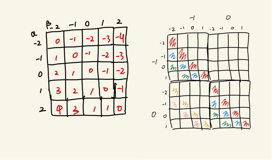
Equation ($\ref{eq:4}$) is easier to understand in the 1D case, where $\mathbf{P}_{(c,\alpha), (d, \beta)}$ just simply contructs a matrix and $\mathbf{K}_{c,d}(m)$ is the sum of its m-th diagonal. A similar conclusion can be drawn in the 2D case by flattening the 2D array into 1D vectors: first compute the sum of the diagonals of each block matrix, and then sum these results according to the second index. The figure below illustrates this procedure, where elements of the same color belong to the same $m$-index. The time complexity is nearly $O(N_z^2N_y^2N_x^2 + N_z^2(2N_x-1)N_y^2 + (2N_x-1)(2N_y-1)N_z^2)$.

The code snippet below shows how this is implemented in Python:
import numpy as np

def sum_of_diags(A, axis1=-2, axis2=-1, L2R=True):
    """Compute the sum of diagonals of a matrix

    Parameters
    ----------
    A : array_like
        Input matrix of shape (..., M, ..., M, ...).
    axis1 : int, optional
        First axis to sum over. Default is -2.
    axis2 : int, optional
        Second axis to sum over. Default is -1.
    L2R: bool, optional
        If True, the sums of diagonals are computed from the left bottom to the
        right top, else the sums of diagonals are computed from the right top to the
        left bottom. Default is True.

    Returns
    -------
    B : array_like
        The sum of the diagonals and subdiagonals of A, with shape (..., 2 * M - 1, ...)
        Values are put along the axis2, from the right top to the left bottom.
    """
    Ndim = A.ndim
    if Ndim < 2:
        raise ValueError("A must be at least 2-dimensional.")
    if A.shape[axis1] != A.shape[axis2]:
        raise ValueError("The two dimensions of A must be equal.")
    M = A.shape[axis2]
    new_shape = list(np.shape(A))
    new_shape[axis2] = 2 * M - 1
    del new_shape[axis1]

    B = np.zeros_like(A, shape=tuple(new_shape))
    flag = 1 if L2R else -1
    for i in range(-M + 1, M):
        new_indices = [
            slice(None) if j != np.mod(axis2, Ndim) else i + M - 1 for j in range(Ndim)
        ]
        del new_indices[axis1]
        B[tuple(new_indices)] = np.trace(A, offset=flag * i, axis1=axis1, axis2=axis2)

    return B
This trick even reduces memory consumption by a factor of 3 with a 2D input.
Phase Ambiguity Problem
As shown in Equation ($\ref{eq:1}$), an arbitrary phase can be applied to the same pair of singular vectors or eigenvector. A simple way to resolve this phase ambiguity problem is to substract the phase of each coil sensitivity map relative to that of the first map. However, this approach also forces the phase of the first map to zero, which can sometimes cause problems in MRI reconstruction.
An alternaive to using the first map as a reference is to subtract the phases relative to that of the first principle component of the coils. This approach is also the default setting of the ecalib command in BART. The rotation matrix can be obtained by a simple coil compression method, which is essentially a PCA of the calibartion data. After completing the whole ESPIRiT procedure, a reference map is extracted using the first column of the rotation matrix, leaving the arbitrary phases unchanged. By subtracting the phase of this reference map, the arbitrary phases can also be canceled out.
However, both methods change the phase distribution of coil sensitivity maps. Uecker and Lustig proposed VCC-ESPIRiT to esitimate actual phase maps of coils. This approach utilizes the conjugate symmetric property of Fourier transform:
\[\begin{equation} \begin{split} y_c(\vec{k}) &= \int x(\vec{r}) B_{c}(\vec{r}) e^{-i 2 \pi \vec{k}\cdot\vec{r}}d\vec{r}\\ y_c(-\vec{k})^* &= \int x(\vec{r}) B_{c}^*(\vec{r}) e^{-i 2 \pi \vec{k}\cdot\vec{r}}d\vec{r} \end{split} \end{equation}\]where $B_{c}(\vec{r})$ is the $c$-th coil sensitivity map at the location $\vec{r}$ and $x(\vec{r})$ is a real-valued pixel of the image. This implies that we could extent the original calibration data by flipping and conjugating the original one:
\[\begin{equation} \begin{split} [y_1(\vec{k}),\cdots,y_{N_c}(\vec{k}),y_1^*(-\vec{k}),\cdots,y_{N_c}^*(-\vec{k})] \end{split} \end{equation}\]Then we can theorectically obtain coil sensitivity maps with ESPIRiT, except for an unkown phase $\theta_r$ across all channels:
\[\begin{equation} \begin{split} &[\hat{B}_{1}(\vec{r}),\cdots,\hat{B}_{N_c}(\vec{r}),\hat{B}_{1}^*(\vec{r}),\cdots,\hat{B}_{N_c}^*(\vec{r})] =\\ &e^{i\theta_r}[B_{1}(\vec{r}),\cdots,B_{N_c}(\vec{r}),B_{1}^*(\vec{r}),\cdots,B_{N_c}^*(\vec{r})] \end{split} \end{equation}\]which can be estimated by:
\[\begin{equation} \begin{split} \frac{1}{2} Imag[ \log \sum_{i=1}^{N_c} \hat{B}_{i}(\vec{r}) \hat{B}_{i}^*(\vec{r}) ] &= \theta_r + n \pi,\ n \in \mathbb{Z} \end{split} \end{equation}\]Substracting this estimated phase leaves only the sign ambiguity $e^{-in\pi}$, which can be resolved by aligning with a low-resolution phase map extracted from the calibration data, ensuring consistency in the sign of the real part.
I still don’t fully understand this alignment step from the offical repo. It seems they rotated the low-resolution phase map by 90 degrees for the second map, but there’s no comment explaining why.
To be honest, the BART documentation is extremly poor. I can’t imagine such a large project having almost no API documentation. The only resources you can rely on are their webinars. Many details are buried in the source code, and you have to dig through it yourself to find them. They don’t even explain the most basic rules, like dimension ordering, in the most obvious places on their website.
But I’m just trying to understand how a few commands work—I can’t be expected to watch dozens of hours of webinars just to figure that out.
In contrast, Numpy’s documentation is extremely user-friendly.
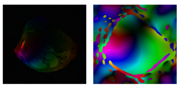
VCC-ESPIRiT retrieves coil sensitivity phase maps with doubling the channels, but at higher computational and memory cost. The sign alignment procedure is also not perfect.

Determine the Dimension of Null Space
The dimension of the null space of $\mathbf{A}$ is estimated by applying a threshold relative to the maximum singular value; Singular values exceeding this threshold are considered belonging to the row space of $\mathbf{A}$. The number of these singular values is $N_k$, as defined earlier.