Dive into ESPIRiT, from Theory to Practice
This post summarizes the ESPIRiT algorithm for estimating coil sensitivies in MRI. It took me months to grasp the theory behind it.
A short introduction
MRI is a common imaging technique for medical diagnosis nowadays. It’s nearly harmless for humans in contrast to other radioactive imaging techniques. In MRI, when a patient is exposed to a magnetic field, hydrogen atoms align with the field. This alignment could be disrupt by a radiofrequency pulse. As the atoms return to their original alignment, they emit signals captured by sensors and used to create medical images.
The signals captured by a sensor $c$ (or coil $c$) can be approximately formulated as:
\[\begin{equation} \begin{split} y_c(\vec{k}(t)) = \int x(\vec{r}) B_{c}(\vec{r}) e^{-i 2 \pi \vec{k}(t)\cdot\vec{r}}d\vec{r} \end{split} \end{equation}\]where $x(\vec{r})$ is an unkown tissue value at location $\vec{r}$, $B_{c}(\vec{r})$ is some value related to the receiver coil $c$, often named as coil sensitivities, $\vec{k}(t)$ is k-space coordinates along with the time $t$. It’s common to have dozens of coils in clinical settings.
This formula indicates that the signals captured by the coil $c$ are fourier transform of interested tissue values which are multipled by the sensitivity map of the coil $c$. A concise way of the above formula is to represent it with operators:
\[\begin{equation} \begin{split} y_c = \mathcal{F}\mathcal{S}_cx \end{split} \end{equation}\]where $\mathcal{F}$ denotes fourier transform, $\mathcal{S}_c$ denotes the sensitivity map of the coil $c$, $y_c$ and $x$ are both vectorized.
Most of the time, coil sensitivities are not available beforehand. We have to estimate them from acquired signals. ESPIRiT is such a method for estimating coil sensitivities , supported by soild theoretical analysis.
About GRAPPA
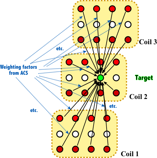
Before diving into ESPIRiT, it’s important to first understand GRAPPA, a well-established parallel imaging method used in MRI. The core of GRAPPA is to interpolate missing k-space points by linearly weighting neighboring acquired points, with the weighting coefficients determined from the calibration region.
Again, a concise way to describe GRAPPA is using operators:
\[\begin{equation} \begin{split} x_c(r) = (\mathcal{P}_{k}\mathcal{R}_ry)^T \mathbf{g}_{c} \end{split} \end{equation}\]where $y$ represents the vectorized multicoil k-space data with unacquired data set to zero, $x_c(r)$ is the estimated value for coil $c$ at location $r$ (for simplicity, the vector notation is omitted, but keep in mind that $r$ is a discrete spatial vector index), $\mathbf{g}_c$ denotes weighting coefficients for coil $c$, $\mathcal{R}_r$ is a patch operator that selects a local block of data around location $r$ and $\mathcal{P}_k$ is a sampling operator that selects only the acquired points within the patch (the subscript $k$ implies that there may exist many sampling patterns).
We can easily construct linear equations using the data from the calibration region, with the same undersamping pattern $\mathcal{P}_k$:
\[\begin{equation} \begin{split} \mathbf{y}_c^{AC} = \mathbf{A}\mathcal{P}_k^T\mathbf{g}_c \end{split} \end{equation}\]where $\mathbf{y}_c^{AC}$ denotes the vectorized data in the calibration region, $\mathbf{A}$ is a so-called calibration matrix, that each row is a local patch around the current acquired point. In this case, $\mathbf{g}_c$ can be efficiently solved by many numerical methods.
By construction , one of the columns of $\mathbf{A}$ is actually $\mathbf{y}_c^{AC}$ itself. Write this as $\mathbf{A}\mathbf{e}_c = \mathbf{y}_c^{AC}$, where $\mathbf{e}_c$ is a vector with 1 in the appropriate location to select the corresponding column of $\mathbf{A}$. We note that:
\[\begin{equation} \begin{split} \mathbf{A}\mathcal{P}_k^T\mathbf{g}_c - \mathbf{y}_c^{AC} &= 0\\ \mathbf{A}\mathcal{P}_k^T\mathbf{g}_c - \mathbf{A}\mathbf{e}_c &= 0\\ \mathbf{A}(\mathcal{P}_k^T\mathbf{g}_c - \mathbf{e}_c) &= 0 \end{split} \end{equation}\]The existence of null-space implies redundancy in row-space of $\mathbf{A}$. $\mathbf{g}_c$ in GRAPPA are very specific null-space vectors. Instead of using this specific form, ESPIRiT analyzes the calibration matrix $\mathbf{A}$ directly.
Key assumptions in ESPIRiT
Since the matrix $\mathbf{A}$ is constructed using local patches in the calibration region, ESPIRiT assumes that all patches, whether in the calibration region or not, lie in the row-space of $\mathbf{A}$:
\[\begin{equation} \begin{split} \mathbf{V}_{\perp}^T\mathcal{R}_r \mathbf{x} &= \mathbf{0}, \quad \forall r \end{split} \end{equation}\]where $\mathbf{V}_{\perp}$ is the basis that spans the null-space and $\mathbf{x}$ is the vectorized multicoil k-space data. Note that “lying in the row-space” is equivalent to being orthogonal to the null-space.
I wrote the formula as $\mathbf{V}_{\perp}^H\mathcal{R}_r \mathbf{x}$, following the same notation used in the paper. However, this ultimatley leads to an algorithm that conflicts with most correct implementations, which require flipping the kernels before applying the Fourier transform. Neither the paper nor subsequent research discussed this operation in detail. This confused me for months and it was truly frustrating.
I think the mismatch arises from how we handle the inner product of complex vectors. The rows of the matrix A are flattened row vectors extracted from local patches $(\mathcal{R}_r \mathbf{x})^T$. However, the standard Hermitian inner product is defined for column vectors. That’s to say, we should use compute the inner product of $\mathbf{V}_{\perp}$ and $((\mathcal{R}_r \mathbf{x})^T)^H$ which is $(\mathbf{V}_{\perp}^T\mathcal{R}_r \mathbf{x})^*$ instead of $\mathbf{V}_{\perp}^H\mathcal{R}_r \mathbf{x}$ from the original paper. The conjugate symbol can be discarded.
$\mathbf{V}_{\perp}$ is computed by singular value decomposition of $\mathbf{A}$: \(\begin{equation} \begin{split} \mathbf{A} &= \mathbf{U} \mathbf{\Sigma} \mathbf{V}^H\\ &= \mathbf{U} \mathbf{\Sigma} \begin{bmatrix} \mathbf{V}_{\parallel} & \mathbf{V}_{\perp} \end{bmatrix}^H \end{split} \end{equation}\)
where $\mathbf{V}_{\parallel}$ corresponds to non-zero singular values and $\mathbf{V}_{\perp}$ corresponds to zero singular values.
Solving the nullspace constraint in the least-square framework
\[\DeclareMathOperator*{\argmin}{arg\,min} \begin{equation} \begin{split} \argmin_{\mathbf{x}} \quad \sum_{r} \frac{1}{2} \|\mathbf{V}_{\perp }^T \mathcal{R}_r \mathbf{x}\|_F^2 \end{split} \label{eq:9} \end{equation}\]which leads to the following equations by zeroing out the gradient:
\[\begin{equation} \begin{split} \sum_r \mathcal{R}_r^H\left(\mathbf{V}_{\perp}\mathbf{V}_{\perp}^H\right)^*\mathcal{R}_r\mathbf{x} = \mathbf{0} \end{split} \end{equation}\]Since $\mathbf{V}$ is unitary, we have $\mathbf{I} = \mathbf{V}_{\perp}\mathbf{V}_{\perp}^H + \mathbf{V}_{\parallel}\mathbf{V}_{\parallel}^H$. By substituting into the above equations, we get:
\[\begin{equation} \begin{split} \sum_r \mathcal{R}_r^H\left(\mathbf{V}_{\parallel}\mathbf{V}_{\parallel}^H\right)^*\mathcal{R}_r\mathbf{x} = \sum_r \mathcal{R}_r^H\mathcal{R}_r \mathbf{x} \end{split} \end{equation}\]The effect of $\mathcal{R}_r^H\mathcal{R}_r$ is to restore the patch to its original location while zeroing out others elements. The overall effect of $\sum_r \mathcal{R}_r^H\mathcal{R}_r$ is a diagonal matrix, where each diagonal element equals to $M$, indicating the number of times it appears in the neighboring patches. With $M$, the equation can be transformed to:
\[\begin{equation} \begin{split} M^{-1}\sum_r \mathcal{R}_r^H\left(\mathbf{V}_{\parallel}\mathbf{V}_{\parallel}^H\right)^*\mathcal{R}_r\mathbf{x} = \mathbf{x} \end{split} \end{equation}\]which is equation (\ref{eq:9}) in the paper except for the conjugation.
“Obvious” convolution
The most challenging part for me is to derive equation (16) $\mathcal{G}_q \vec{s}_q = \vec{s}_q$ from the paper. The authors mentioned that the operator $\mathcal{W} = M^{-1}\sum_r \mathcal{R}_r^H\mathbf{V}_{\parallel}\mathbf{V}_{\parallel}^H\mathcal{R}_r$ (in our case, $\mathcal{W} = M^{-1}\sum_r \mathcal{R}_r^H\left(\mathbf{V}_{\parallel}\mathbf{V}_{\parallel}^H\right)^*\mathcal{R}_r$) is a matrix-valued convolution, which can be decoupled into point-wise matrix operations in the image domain. The sensitivity maps are obtained by the eigenvalue decomposition of all $\mathcal{G}_q$'s choosing only the eigenvectors corresponding to eigenvalue "=1".
The intutive is that we could use the Fourier Convolution Theorem to get what we want, which is more straightforward in scalar cases. However, since $\mathcal{W}$ is a high-dimensional operator (k-space locations and channels), applying the theorem directly is not straightforward. A better approach would be to transform $\mathcal{W}$ into a form that resembles something familiar in 1D.
To simplify the derivation, we first introduce some notations:
- $\mathbf{P} =\left(\mathbf{V}_{\parallel}\mathbf{V}_{\parallel}^H\right)^*$: $\mathbf{P}$ operates on patches
- $\mathbf{P}_{(c,\alpha), (d, \beta)}$: a scalar value, where $(c,\alpha)$ represents the c-th channel and location $\alpha$ in the output (row index), and $(d, \beta)$ represents the $d$-th channel and location $\beta$ in the input (column index)
- $\mathbf{x}_c(r)$: a scalar value, where $c$ represents the $c$-th channel and $r$ reprsents location $r$ in the k-space
- $(\mathcal{R}_r\mathbf{x})_{(d, \beta)}$: a scalar value, the $d$-th coil value at location $\beta$ in the patch centered at location $r$
- $(\mathbf{P}\mathcal{R}_r\mathbf{x})_{(c,\alpha)}$: a scalar value, the $c$-th coil value at location $\alpha$ of the output
- $(\mathcal{R}_r^H\mathbf{P}\mathcal{R}_r\mathbf{x})_c(m)$: a scalar value, the $c$-th coil value at location $m$ in the k-space
As we have discussed above, $\mathcal{R}_r$ extracts a patch centered at location $r$:
\[\begin{equation} \begin{split} (\mathcal{R}_r\mathbf{x})_{(d,\beta)}=\mathbf{x}_d(r+\beta) \end{split} \end{equation}\]where $\beta$ represents the relative shift with respect to the central location $r$.
The effect of $\mathbf{P}$ is to perform a weighted summation across the channels and locations of the input:
\[\begin{equation} \begin{split} (\mathbf{P}\mathcal{R}_r\mathbf{x})_{(c,\alpha)} &= \sum_{d,\beta}\mathbf{P}_{(c,\alpha), (d, \beta)} (\mathcal{R}_r\mathbf{x})_{(d,\beta)}\\ &= \sum_{d,\beta}\mathbf{P}_{(c,\alpha), (d, \beta)}\mathbf{x}_d(r+\beta) \end{split} \end{equation}\]The effect of $\mathcal{R}_r^H$ is to restore the patch to its original location while zeroing out others elements:
\[\begin{equation} \begin{split} (\mathcal{R}_r^H\mathbf{P}\mathcal{R}_r\mathbf{x})_c(m) &= \sum_{\alpha} \delta(m, r+\alpha)(\mathbf{P}\mathcal{R}_r\mathbf{x})_{(c,\alpha)} \end{split} \end{equation}\]where $\delta(\cdot, \cdot)$ is the Kronecker delta function, which plays an important role in eliminating the inner $\alpha$.
With these notations, we have:
\[\begin{equation} \begin{split} (\mathcal{W}\mathbf{x})_c(m) &= M^{-1}\sum_r (\mathcal{R}_r^H\mathbf{P}\mathcal{R}_r\mathbf{x})_c(m)\\ &= M^{-1}\sum_r\sum_{\alpha} \delta(m, r+\alpha)(\mathbf{P}\mathcal{R}_r\mathbf{x})_{(c,\alpha)}\\ &= M^{-1}\sum_r\sum_{\alpha} \delta(m, r+\alpha)\sum_{d,\beta}\mathbf{P}_{(c,\alpha), (d, \beta)}\mathbf{x}_d(r+\beta)\\ &=M^{-1}\sum_{\alpha,d,\beta}\sum_r\delta(m, r+\alpha)\mathbf{P}_{(c,\alpha), (d, \beta)}\mathbf{x}_d(r+\beta) \end{split} \end{equation}\]Since $\delta(m,r+\alpha) = 1$ if and only if $m=r+\alpha$, we further have:
\[\begin{equation} \begin{split} (\mathcal{W}\mathbf{x})_c(m) &= M^{-1}\sum_{\alpha,d,\beta}\mathbf{P}_{(c,\alpha), (d, \beta)}\mathbf{x}_d(m - (\alpha-\beta)) \end{split} \end{equation}\]Let $u=\alpha - \beta$ represents the difference between the relative shifts, then:
\[\begin{equation} \begin{split} (\mathcal{W}\mathbf{x})_c(m) &= M^{-1}\sum_{d} \sum_u (\sum_{\alpha,\beta,\alpha - \beta= u}\mathbf{P}_{(c,\alpha), (d, \beta)})\mathbf{x}_d(m - u)\\ &=M^{-1}\sum_{d} \sum_u \mathbf{K}_{c,d}(u)\mathbf{x}_d(m - u) \end{split} \label{eq:18} \end{equation}\]where $\mathbf{K}_{c,d}(u) = \sum_{\alpha,\beta,\alpha - \beta= u}\mathbf{P}_{(c,\alpha), (d, \beta)}$. Recall that $u$ is determined by the relative shifts of $\alpha$ and $\beta$. What we are doing here is actually re-grouping the pairs $(\alpha, \beta)$ according to their common difference $u$. We don't need to worry about how to compute $\mathbf{K}_{c,d}(u)$ right now; we only need to understand that it is a scalar value associated with $c,d$ and the difference $u$.
Finally, we got something that looks like a convolution. $\sum_u \mathbf{K}_{c,d}(u)\mathbf{x}_d(m - u)$ is a convolution of $\mathbf{K}_{c,d}(m)$ and $\mathbf{x}_d(m)$. It's worth noting that $u$ cannot exceed twice the size of the patch, as it represents the difference between the relative shifts. $\mathbf{K}_{c,d}(m)$ is only meaningful in this range.
Calculate coil sensitivies
We should know that $\mathbf{x}_c(m)=\mathcal{F}[\mathbf{s}_c(n)\hat{\mathbf{x}}(n)](m)$, as we have discussed in the introduction. Let's add it to the right-hand side of the equation:
\[\begin{equation} \begin{split} (\mathcal{W}\mathbf{x})_c(m) &= \mathbf{x}_c(m)\\ M^{-1}\sum_{d} \mathbf{K}_{c,d}(m) \ast\mathbf{x}_d(m) &= \mathbf{x}_c(m)\\ \end{split} \end{equation}\]Apply the inverse Fourier transform on both sides:
\[\begin{equation} \begin{split} M^{-1}\sum_{d} \hat{\mathbf{K}}_{c,d}(n)\mathbf{s}_d(n)\hat{\mathbf{x}}(n) &= \mathbf{s}_c(n)\hat{\mathbf{x}}(n)\\ \end{split} \end{equation}\]where $\hat{\mathbf{x}}(n)$ is in image-space, $\mathbf{s}_d(n)$ is the $d$-th coil sensitivity value at the location $n$. With all coils at the location $n$, we have:
\[\begin{equation} \begin{split} M^{-1} \begin{bmatrix} \hat{\mathbf{K}}_{1,1}(n) & \cdots & \hat{\mathbf{K}}_{1,N_c}(n)\\ \vdots & \ddots & \vdots\\ \hat{\mathbf{K}}_{N_c,1}(n) & \cdots & \hat{\mathbf{K}}_{N_c,N_c}(n)\\ \end{bmatrix} \begin{bmatrix} \mathbf{s}_1(n)\\ \vdots\\ \mathbf{s}_{N_c}(n)\\ \end{bmatrix} \hat{\mathbf{x}}(n) &= \begin{bmatrix} \mathbf{s}_1(n)\\ \vdots\\ \mathbf{s}_{N_c}(n)\\ \end{bmatrix} \hat{\mathbf{x}}(n) \end{split} \label{eq:21} \end{equation}\]where $\hat{\mathbf{x}}(n)$ can be eliminated if it is non-zero.
Now it’s clear that the coil sensitivities at location $n$ are the eigenvectors corresponding to the eigenvalues equal to 1.
The remaining question is what the inverse Fourier transform of $\hat{\mathbf{K}}_{c,d}(n)$ is:
\[\begin{equation} \begin{split} \hat{\mathbf{K}}_{c,d}(n) &= \frac{1}{N}\sum_m \mathbf{K}_{c,d}(m) e^{i2\pi\frac{nm}{N}}\\ &= \frac{1}{N} \sum_m \sum_{\alpha,\beta,\alpha - \beta= m}\mathbf{P}_{(c,\alpha), (d, \beta)} e^{i2\pi\frac{nm}{N}}\\ &= \frac{1}{N} \sum_{\alpha,\beta}\mathbf{P}_{(c,\alpha), (d, \beta)} e^{i2\pi\frac{n(\alpha-\beta)}{N}}\\ \end{split} \end{equation}\]where $N$ is the number of spatial locations. Here we eliminate $m$ by re-grouping elements according to the $\alpha$ and $\beta$. Recall that $\mathbf{P} =\left(\mathbf{V}_{\parallel}\mathbf{V}_{\parallel}^H\right)^*$:
\[\begin{equation} \begin{split} \mathbf{P}_{(c,\alpha), (d, \beta)} &= \sum_k \mathbf{v}_k^*(c,\alpha)\mathbf{v}_k(d,\beta) \end{split} \end{equation}\]where $\mathbf{v}_k(c,\alpha)$ represents a scalar value of the coil $c$ and location $\alpha$ of the $k$-th component of $\mathbf{V}_{\parallel}$. Then we have:
\[\begin{equation} \begin{split} \hat{\mathbf{K}}_{c,d}(n) &= \frac{1}{N} \sum_{\alpha,\beta}\mathbf{P}_{(c,\alpha), (d, \beta)} e^{i2\pi\frac{n(\alpha-\beta)}{N}}\\ &= N \sum_k \left(\frac{1}{N} \sum_{\alpha} \mathbf{v}_k^*(c, \alpha)e^{i2\pi\frac{n\alpha}{N}}\right)\left(\frac{1}{N} \sum_{\beta} \mathbf{v}_k(d, \beta)e^{-i2\pi\frac{n\beta}{N}}\right)\\ &= N \sum_k \hat{\mathbf{v}}_k(c, n)\hat{\mathbf{v}}_k^*(d, n) \end{split} \label{eq:24} \end{equation}\]where $\hat{\mathbf{v}}_k(c, n)$ is the inverse Fourier transform of the conjugated $\mathbf{v}_k(c, m)$ at the location $n$.
Substituting equation (\ref{eq:24}) into equation (\ref{eq:21}):
\[\begin{equation} \begin{split} \mathbf{G}_n \mathbf{G}_n^H \begin{bmatrix} \mathbf{s}_1(n)\\ \vdots\\ \mathbf{s}_{N_c}(n)\\ \end{bmatrix} &= \begin{bmatrix} \mathbf{s}_1(n)\\ \vdots\\ \mathbf{s}_{N_c}(n)\\ \end{bmatrix} \end{split} \end{equation}\]where $\mathbf{G}_n = M^{-1/2}N^{1/2}\begin{bmatrix} \hat{\mathbf{v}}_1(1, n) & \cdots & \hat{\mathbf{v}}_{N_k}(1, n)\\ \vdots & \ddots & \vdots\\ \hat{\mathbf{v}}_1(N_c, n) & \cdots & \hat{\mathbf{v}}_{N_k}(N_c, n)\\ \end{bmatrix}$.
Let’s summarize the steps to compute coil sensitivities:
- Reshape $\mathbf{V}_{\parallel}$ to the shape $M \times N_c \times N_k$
- Center it and pad it to the full-grid size $N \times N_c \times N_k$
- Apply the inverse Fourier transform on the conjugated k-space kernels
- Extract $\mathbf{G}_n$ of shape $N_c \times N_k$ for each pixel $n$
- Compute eigenvectors of $\mathbf{G}_n\mathbf{G}_n^H$
- Select the eigenvectors corresponding to the eigenvalues of 1, which represent the coil sensitivities at pixel $n$
- Repeat 4 to 6 until all pixels have been processed
Connections to the “kernel flippling” operation
Most implementations would do the following kernel flipping operation before applying the Fourier transform:
KERNEL = zeros(imSize(1), imSize(2), size(kernel,3), size(kernel,4));
for n=1:size(kernel,4)
    KERNEL(:,:,:,n) = (fft2c(zpad(conj(kernel(end:-1:1,end:-1:1,:,n))*sqrt(imSize(1)*imSize(2)), ...
        [imSize(1), imSize(2), size(kernel,3)])));
end
Instead, our algorithm suggests that:
KERNEL = zeros(imSize(1), imSize(2), size(kernel,3), size(kernel,4));
for n=1:size(kernel,4)
    KERNEL(:,:,:,n) = (ifft2c(zpad(conj(kernel)*sqrt(imSize(1)*imSize(2)), ...
        [imSize(1), imSize(2), size(kernel,3)])));
end
By using the shift properties of the Fourier transform, We can show that:
\[\begin{equation} \begin{split} ifft(ifftshift(x))[m] = e^{i2\pi \frac{m}{N} (2\lceil N/2\rceil -1)} fft(ifftshift(x^*_{rev})) \end{split} \end{equation}\]where $x^*_{rev}$ is the conjugate of the reversed signal $x$. If $N$ is odd, our implementation is equivalent to the kernel flipping operation. However, if $N$ is even, there exists a linear phase term $e^{-i2\pi \frac{m}{N}}$ between the two methods.
I am still investigating the differences between the two methods. However, based on the assumptions in the original paper, I ended up with algorithmic steps that, for unknown reasons, do not match those in other offical implementaions such as bart.
I believe Professor Haldar’s linear-predictability framework may help explain the discrepancy here. In that work, the authors present a connection between ESPIRiT and the nullspace algorithm direclty, but without providing a proof. Surprisingly, one of their acceleration techniques(Section IV, Part C) is quite similar to my relative shift trick in equation (18). I plan to explore the underlying mathematical relationships in my following posts.